import ...`); the card links to the full source and to the page of the user guide which explains the method.
- __Timecourses__
---
[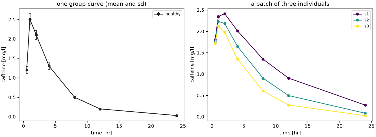](images/timecourses.png)
One curve with its dose, its units and the uncertainty of a group, and a batch of several curves over the sample dimensions.
```python
from pkpdutils import Dose, Route, Timecourse
tc = Timecourse(
time=[0.5, 1, 2, 4, 8, 12, 24],
value=[1.2, 2.5, 2.1, 1.3, 0.5, 0.2, 0.03],
sd=[0.3, 0.5, 0.4, 0.3, 0.1, 0.05, 0.01],
n=12,
time_unit="hr",
unit="mg/l",
dose=Dose(amount=100, unit="mg", route=Route.ORAL),
)
```
[timecourses.py](https://github.com/matthiaskoenig/pkpdutils/blob/develop/examples/timecourses.py) · [Timecourses](timecourses.md)
- __NCA of one curve__
---
[](images/nca_single.png)
[](images/nca_terminal_windows.png)
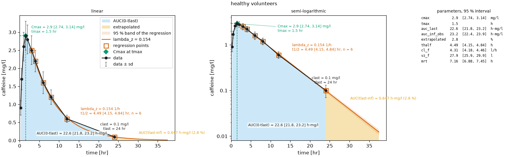
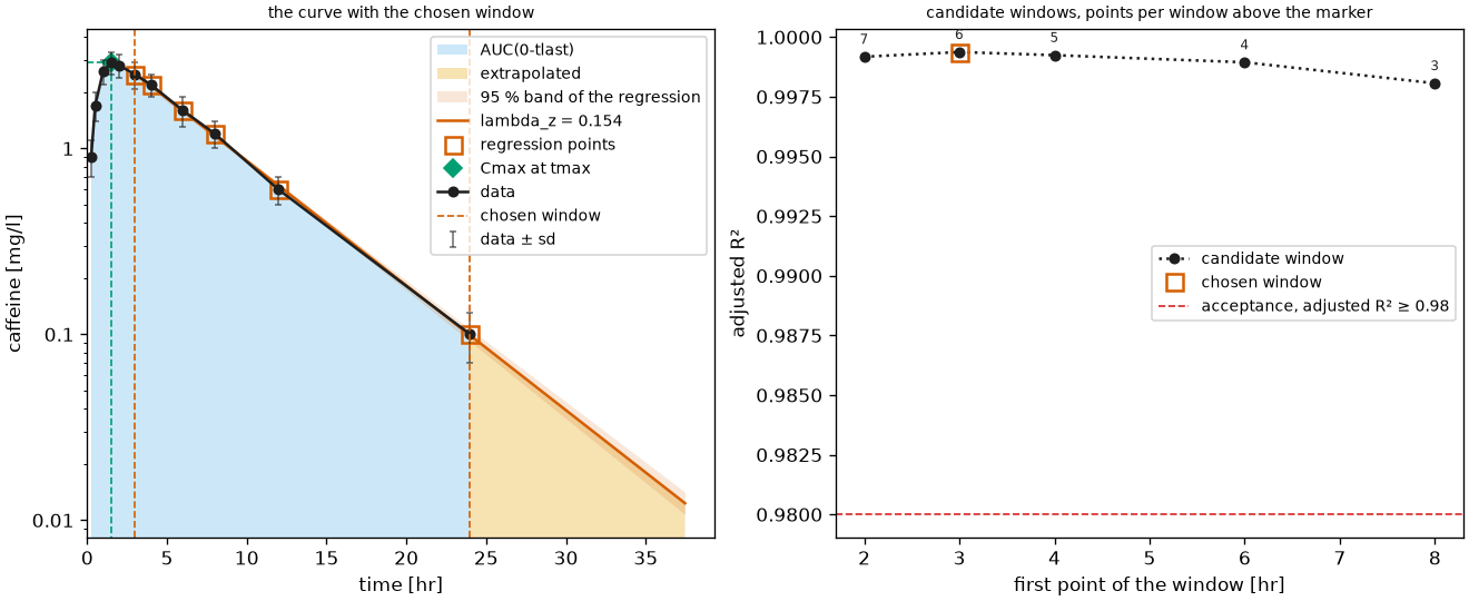
The non-compartmental analysis of a single timecourse with its diagnostic figure: the trapezoidal area, the extrapolated tail, the terminal regression with its confidence band and the parameters with their intervals; and the diagnostic of the terminal phase, every candidate window with its adjusted \(R^2\) and the chosen one marked.
```python
from examples.nca_single import tc
from pkpdutils import Acceptance, NCAOptions, TerminalPhase, nca_single
from pkpdutils.plot import plot_nca, plot_terminal_windows
result = nca_single(tc, options=NCAOptions(seed=1)) # a fixed bootstrap seed
print(result.to_quantities()["auc_inf_obs"])
plot_nca(tc, result).savefig("nca_single.png", dpi=120)
diagnostic = NCAOptions(
terminal=TerminalPhase(keep_candidates=True),
acceptance=Acceptance(r2_adj_min=0.98),
)
windows = nca_single(tc, options=diagnostic)
plot_terminal_windows(tc, windows, options=diagnostic).savefig(
"nca_terminal_windows.png", dpi=120
)
```
[nca_single.py](https://github.com/matthiaskoenig/pkpdutils/blob/develop/examples/nca_single.py) · [Non-compartmental analysis](nca.md)
- __NCA of a batch__
---
[](images/nca_batch_curves.png)
[](images/nca_batch_study.png)
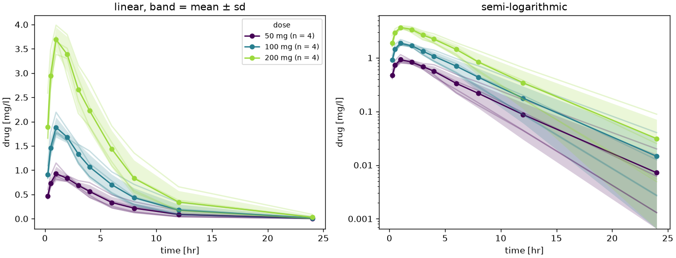
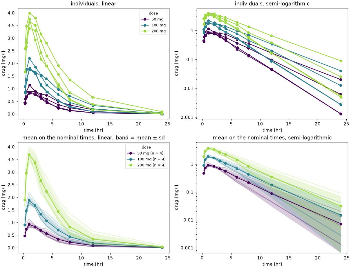
A `(dose, individual)` batch analysed at once: the parameters of every curve as a data frame, the mean curve per dose group, a diagnostic panel per sample and the four panels a study report shows, the individuals on their actual sampling times and the means on the nominal ones.
```python
from examples.nca_batch import batch, study
from pkpdutils import nca
from pkpdutils.plot import plot_mean_timecourse, plot_nca_grid, plot_study_curves
result = nca(batch)
print(result.to_dataframe()[["dose", "individual", "auc_inf_obs", "cmax"]])
plot_mean_timecourse(batch, by="dose").savefig("nca_batch_curves.png", dpi=120)
plot_nca_grid(batch, result, ncols=4).savefig("nca_batch.png", dpi=100)
plot_study_curves(study, by="dose").savefig("nca_batch_study.png", dpi=110)
```
[nca_batch.py](https://github.com/matthiaskoenig/pkpdutils/blob/develop/examples/nca_batch.py) · [Non-compartmental analysis](nca.md)
- __Group uncertainty__
---
[](images/group_uncertainty.png)
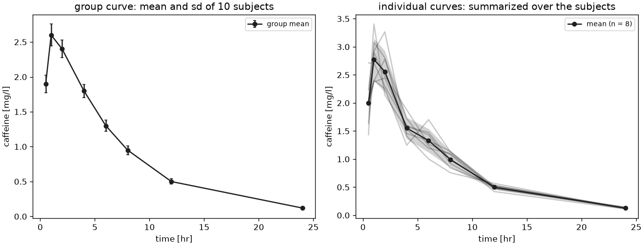
The uncertainty of a published mean curve propagated to the parameters with the bootstrap or the delta method, and individual results summarized over the subjects.
```python
from examples.group_uncertainty import group
from pkpdutils import NCAOptions, nca_single
boot = nca_single(group, options=NCAOptions(seed=1, n_boot=2000))
q = boot.to_quantities()
print(q["auc_inf_obs"], q["auc_inf_obs_ci_low"], q["auc_inf_obs_ci_high"])
```
[group_uncertainty.py](https://github.com/matthiaskoenig/pkpdutils/blob/develop/examples/group_uncertainty.py) · [Uncertainty](uncertainty.md)
- __Multiple dosing and steady state__
---
[](images/steady_state.png)
[](images/steady_state_troughs.png)
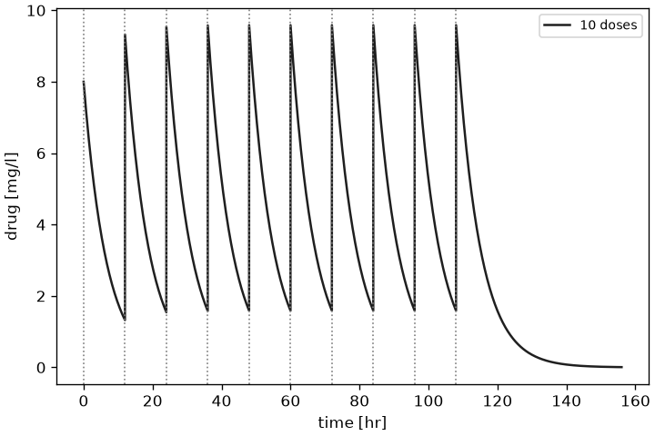
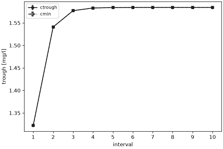
A single dose curve superposed into a regimen of ten doses, the parameters of every dosing interval and the steady state parameters of the last one, with the trough of every interval running into its plateau.
```python
from examples.steady_state import single
from pkpdutils import AUCMethod, Dose, Dosing, NCAOptions, Route, nca_single
from pkpdutils.nca import superposition
from pkpdutils.plot import plot_troughs
dose = Dose(amount=100, unit="mg", route=Route.IV_BOLUS)
protocol = Dosing.regimen(dose, interval=12, n_doses=10)
options = NCAOptions(auc_method=AUCMethod.LOG)
predicted = superposition(single, protocol, options=options)
result = nca_single(predicted, options=options)
print(result.to_quantities()["auc_tau"])
plot_troughs(result, x="interval").savefig("steady_state_troughs.png", dpi=120)
```
[steady_state.py](https://github.com/matthiaskoenig/pkpdutils/blob/develop/examples/steady_state.py) · [Non-compartmental analysis](nca.md)
- __Exchange formats__
---
[](images/formats.png)
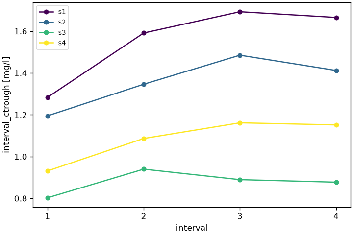
A twice daily batch written as event records and read back, analysed interval by interval; `from_adnca` reads a CDISC ADaM extract the same way.
```python
import pandas as pd
from examples.formats import batch
from pkpdutils import AUCMethod, NCAOptions, Route, Timecourses, nca
from pkpdutils.plot import plot_intervals
batch.to_events().to_csv("events.csv", index=False)
read_back = Timecourses.from_events(
pd.read_csv("events.csv"),
time_unit="hr",
unit="mg/l",
dose_unit="mg",
route=Route.ORAL,
)
result = nca(read_back, options=NCAOptions(auc_method=AUCMethod.LOG))
plot_intervals(result, "interval_ctrough").savefig("formats.png", dpi=120)
```
[formats.py](https://github.com/matthiaskoenig/pkpdutils/blob/develop/examples/formats.py) · [Data formats](formats.md)
- __Exponential fitting__
---
[](images/fitting_exponential.png)
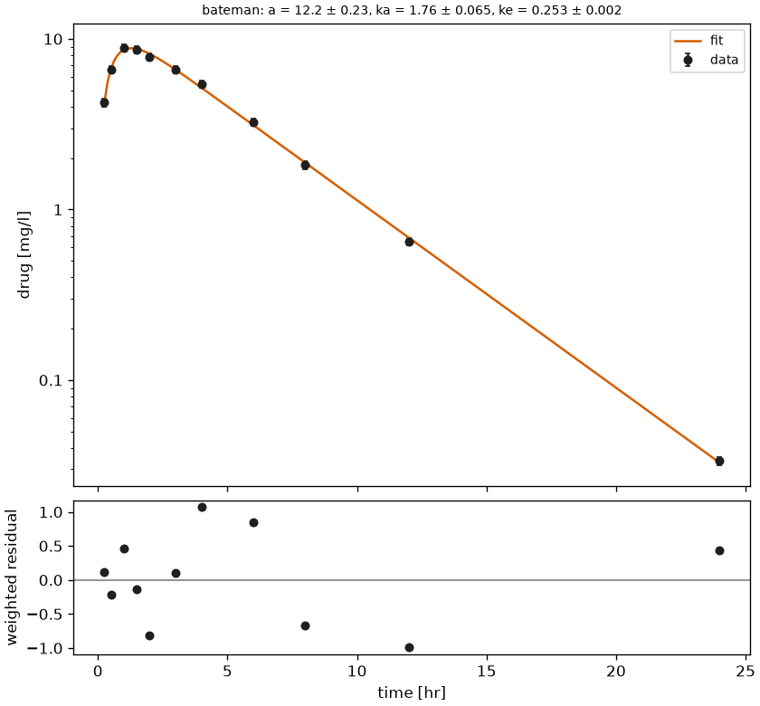
A Bateman model fitted to an oral curve with `1/sd` weighting and a residual bootstrap, and the AICc comparison of the exponential models.
```python
from examples.fitting_exponential import tc
from pkpdutils import Bateman, FitOptions, Weighting, fit_timecourse
from pkpdutils.plot import plot_fit
options = FitOptions(weighting=Weighting.INV_SD, n_starts=5, bootstrap=200, seed=1)
result = fit_timecourse(Bateman(), tc, options=options)
print(result.to_dataframe().T)
plot_fit(result, log_y=True).savefig("fitting_exponential.png", dpi=120)
```
[fitting_exponential.py](https://github.com/matthiaskoenig/pkpdutils/blob/develop/examples/fitting_exponential.py) · [Curve fitting](fitting.md)
- __Emax__
---
[](images/emax.png)
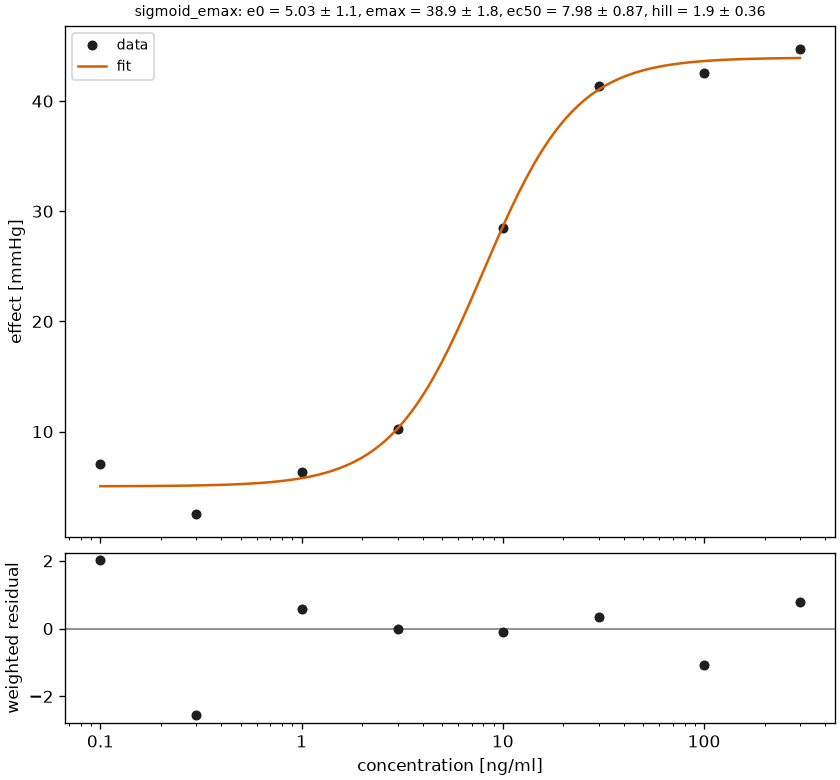
The concentration-effect relationship as a sigmoid Emax model, with `ec50`, `ec90` and the comparison against the Emax and the linear model.
```python
from examples.emax import concentration, effect
from pkpdutils import FitOptions, SigmoidEmax, fit
from pkpdutils.plot import plot_fit
result = fit(
SigmoidEmax(),
concentration,
effect,
x_unit="ng/ml",
y_unit="mmHg",
x_name="concentration",
y_name="effect",
options=FitOptions(n_starts=10, seed=0),
)
print(result.to_quantities()["ec50"])
plot_fit(result, log_x=True).savefig("emax.png", dpi=120)
```
[emax.py](https://github.com/matthiaskoenig/pkpdutils/blob/develop/examples/emax.py) · [Pharmacodynamics](pd.md)
- __Dose proportionality__
---
[](images/dose_proportionality.png)
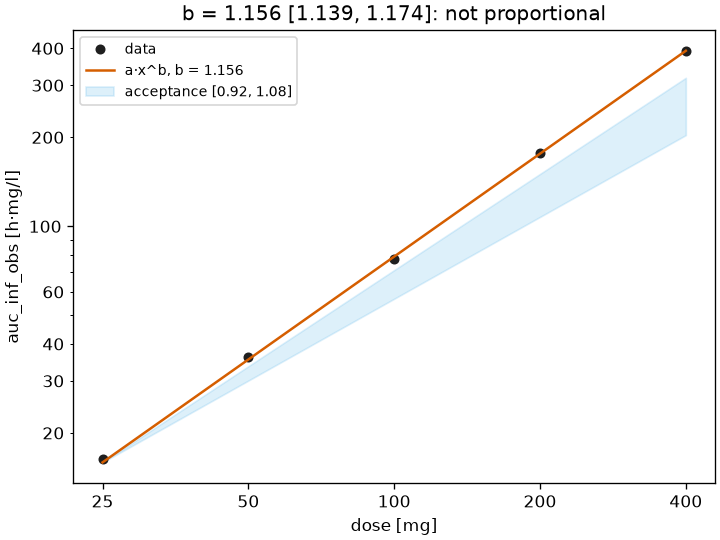
The power model \(AUC = a \cdot dose^b\) over a dose escalation and the confidence interval criterion of the dose proportionality.
```python
from examples.dose_proportionality import batch, doses
from pkpdutils import Power, fit_table, nca, proportionality_test
from pkpdutils.plot import plot_dose_proportionality
result = nca(batch)
ds = result.ds.assign_coords(dose=("dose", doses, {"units": "mg"}))
power = fit_table(Power(), ds, "dose", "auc_inf_obs", dim="dose")
test = proportionality_test(power, dose_range=(25.0, 400.0))
print(test.slope, test.ci_low, test.ci_high, test.proportional)
plot_dose_proportionality(power, test=test).savefig("dose_proportionality.png", dpi=120)
```
[dose_proportionality.py](https://github.com/matthiaskoenig/pkpdutils/blob/develop/examples/dose_proportionality.py) · [Curve fitting](fitting.md)
- __Covariate and allometry__
---
[](images/covariate.png)
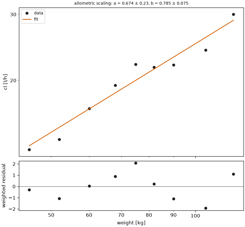
The clearance against the body weight as an allometric model, with a free exponent and with the exponent fixed at 0.75.
```python
from examples.covariate import ds
from pkpdutils import Allometric, fit_table
from pkpdutils.plot import plot_fit
free = fit_table(Allometric(), ds, "weight", "cl", dim="individual")
print(free.to_dataframe().T.loc[["a", "b", "b_ci_low", "b_ci_high"]])
plot_fit(free, log_x=True, log_y=True).savefig("covariate.png", dpi=120)
```
[covariate.py](https://github.com/matthiaskoenig/pkpdutils/blob/develop/examples/covariate.py) · [Curve fitting](fitting.md)
- __Bioequivalence__
---
[](images/bioequivalence.png)
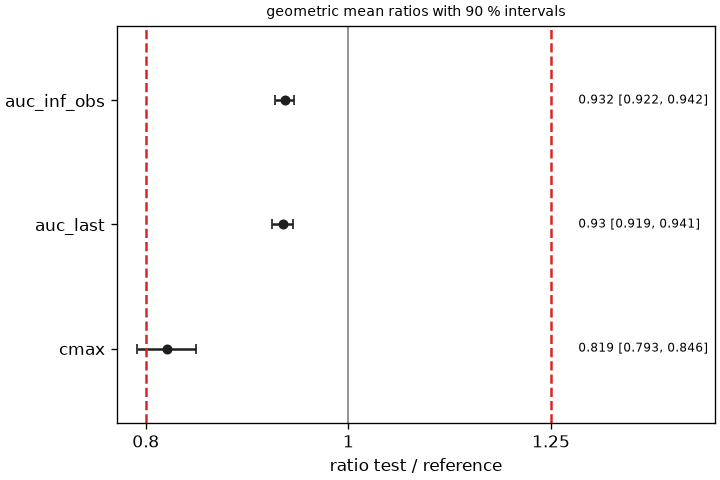
Average bioequivalence of a test against a reference formulation in a 2x2 crossover: the geometric mean ratios with their 90 % intervals against the 80-125 % limits.
```python
from examples.bioequivalence import PERIOD_REF, PERIOD_TEST, batch, curves
from pkpdutils import bioequivalence, nca
from pkpdutils.plot import plot_ratio
reference = nca(batch(curves(1.0, 1.5, PERIOD_REF), PERIOD_REF))
test = nca(batch(curves(0.93, 0.9, PERIOD_TEST), PERIOD_TEST))
result = bioequivalence(test, reference, parameters=["auc_inf_obs", "auc_last", "cmax"])
print(result.to_dataframe()[["parameter", "gmr", "ci_low", "ci_high"]])
plot_ratio(result).savefig("bioequivalence.png", dpi=120)
```
[bioequivalence.py](https://github.com/matthiaskoenig/pkpdutils/blob/develop/examples/bioequivalence.py) · [Statistics](statistics.md)
- __Drug-drug interaction__
---
[](images/ddi.png)
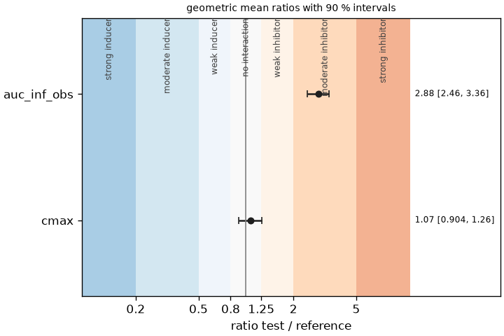
The exposure with and without a perpetrator as a geometric mean ratio, classified against the FDA and EMA thresholds of an interaction.
```python
from examples.ddi import batch
from pkpdutils import ddi_classification, nca, ratio
from pkpdutils.plot import plot_ratio
control = nca(batch(1.0, "control"))
inhibited = nca(batch(0.35, "inhibitor"))
auc = ratio(
inhibited.sample("auc_inf_obs", "individual"),
control.sample("auc_inf_obs", "individual"),
)
print(ddi_classification(auc).to_dict())
plot_ratio({"auc_inf_obs": auc}, limits=None).savefig("ddi.png", dpi=120)
```
[ddi.py](https://github.com/matthiaskoenig/pkpdutils/blob/develop/examples/ddi.py) · [Statistics](statistics.md)
- __Meta-analysis__
---
[](images/meta_analysis.png)
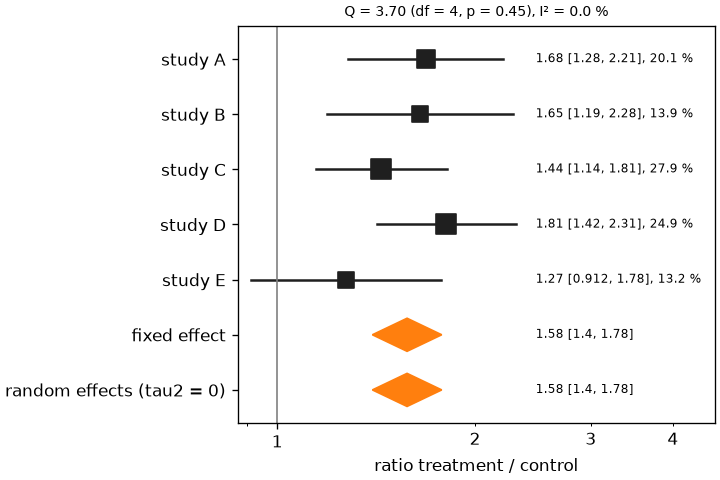
Published summary statistics of several studies pooled with the fixed effect and the random effects model, with the heterogeneity and a forest plot.
```python
from examples.meta_analysis import STUDIES
from pkpdutils import meta_analysis
from pkpdutils.plot import plot_forest
from pkpdutils.stats import EffectKind
result = meta_analysis(STUDIES, EffectKind.LOG_RATIO)
print(result.to_dataframe())
print(result.random.to_dict(), result.heterogeneity.i2)
plot_forest(result).savefig("meta_analysis.png", dpi=120)
```
[meta_analysis.py](https://github.com/matthiaskoenig/pkpdutils/blob/develop/examples/meta_analysis.py) · [Statistics](statistics.md)
- __Simulation scan__
---
[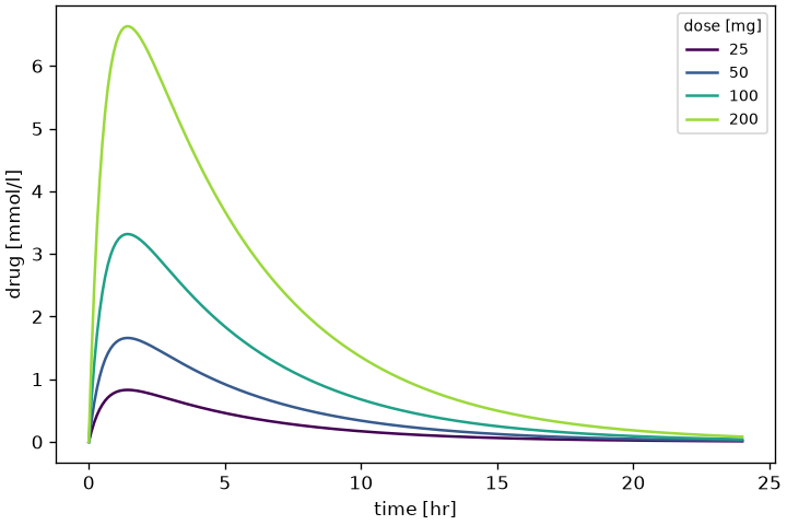](images/nca_from_sbmlsim.png)
The result of a simulation scan read as a batch (`from_dataset`, `from_xresult` for an sbmlsim `XResult`) and analysed curve by curve.
```python
from examples.nca_from_sbmlsim import DOSES, simulated_dataset
from pkpdutils import NCAOptions, Route, Timecourses, nca
from pkpdutils.plot import plot_timecourse
batch = Timecourses.from_dataset(
simulated_dataset(),
"[Cve]",
unit="mmol/l",
time_unit="hr",
dose={"amount": DOSES, "unit": "mg"},
route=Route.ORAL,
)
result = nca(batch, options=NCAOptions())
print(result.to_dataframe()[["dose", "auc_inf_obs", "cmax"]])
plot_timecourse(batch, by="dose").savefig("nca_from_sbmlsim.png", dpi=120)
```
[nca_from_sbmlsim.py](https://github.com/matthiaskoenig/pkpdutils/blob/develop/examples/nca_from_sbmlsim.py) · [Non-compartmental analysis](nca.md)
- __Urinary excretion__
---
[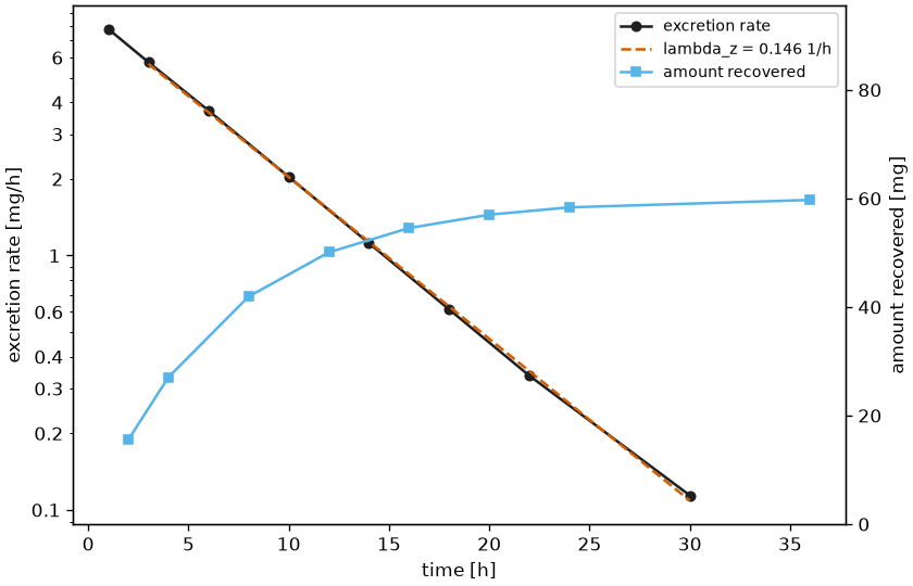](images/urine.png)
The excretion rate of every urine collection against the midpoint of its interval with the terminal regression, and the amount recovered rising to its plateau on a second axis.
```python
from examples.urine import excretion, plasma
from pkpdutils import nca_urine
from pkpdutils.plot import plot_excretion
urine = excretion()
result = nca_urine(urine, plasma=plasma())
print(result.to_quantities()["clr"])
plot_excretion(result, urine).savefig("urine.png", dpi=120)
```
[urine.py](https://github.com/matthiaskoenig/pkpdutils/blob/develop/examples/urine.py) · [Urinary excretion](urine.md)
- __Sparse sampling__
---
[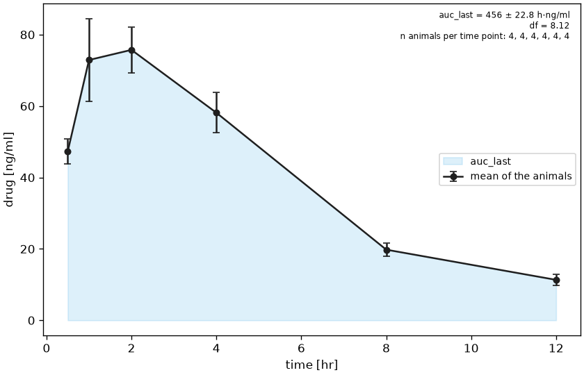](images/sparse.png)
The mean curve of a destructive design with the standard error of every time point, the area the trapezoid rule integrates and the Bailer standard error of that area.
```python
from examples.sparse import TIMES, serial_design
from pkpdutils import nca_sparse, sparse_mean
from pkpdutils.plot import plot_sparse
values = serial_design()
curve = sparse_mean(TIMES, values, time_unit="hr", unit="ng/ml")
result = nca_sparse(TIMES, values, time_unit="hr", unit="ng/ml")
plot_sparse(curve, result).savefig("sparse.png", dpi=120)
```
[sparse.py](https://github.com/matthiaskoenig/pkpdutils/blob/develop/examples/sparse.py) · [Sparse sampling](sparse.md)
- __Study report__
---
[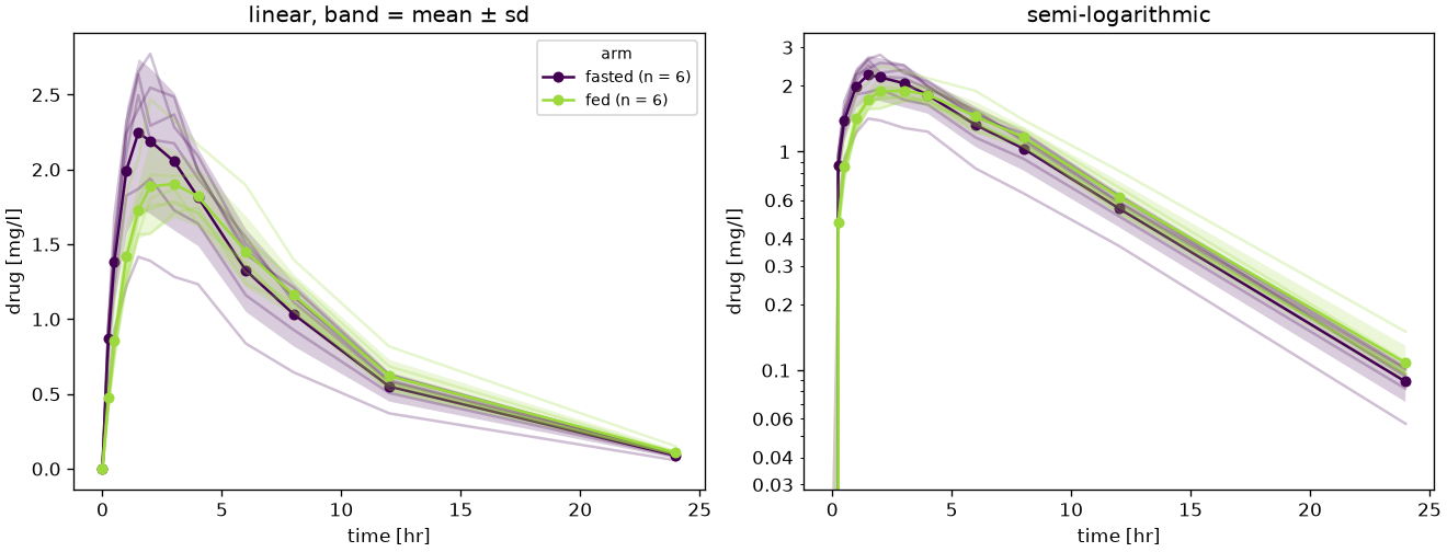](images/report.png)
The tables and the figures of a study assembled into one self-contained HTML document: the methods sentence, the summary statistics of ICH M13A, the acceptability of the extrapolation, the parameters of every subject and the two figures.
```python
from pkpdutils import study_report
report = study_report(batch, result, dim="individual", by="arm")
report.write_html("report.html")
```
[report.py](https://github.com/matthiaskoenig/pkpdutils/blob/develop/examples/report.py) · [Reporting](reporting.md)
---
# Glossary
The names used for the variables of the result datasets, with their symbols and the page that defines them. Units are derived from the units of the input; `value` is the unit of the measured values, `time` the unit of the times, `dose` the unit of the doses.
| name | symbol | meaning | unit | page |
| --- | --- | --- | --- | --- |
| `auc_last` | \(\mathrm{AUC}_{0\text{-}t_\mathrm{last}}\) | area under the curve to the last measurable value | value·time | [NCA](nca.md) |
| `auc_all`, `aumc_all` | \(\mathrm{AUC}_\mathrm{all}\) | area (and moment) to the last observation, the trailing zeros and the values a BLQ rule imputed included | value·time, value·time² | [NCA](nca.md) |
| `auc_inf_obs`, `auc_inf_pred` | \(\mathrm{AUC}_{0\text{-}\infty}\) | area extrapolated to infinity, observed or predicted last value | value·time | [NCA](nca.md) |
| `auc_extrap_fraction` | | extrapolated fraction of \(\mathrm{AUC}_{0\text{-}\infty}\) | – | [NCA](nca.md) |
| `aumc_last`, `aumc_inf` | \(\mathrm{AUMC}\) | area under the first moment curve | value·time² | [NCA](nca.md) |
| `mrt` | \(\mathrm{MRT}\) | mean residence time | time | [NCA](nca.md) |
| `thalf_eff` | \(t_{1/2,\mathrm{eff}}\) | effective half-life, \(\ln 2 \cdot \mathrm{MRT}\) | time | [NCA](nca.md) |
| `cmax`, `tmax` | \(C_\mathrm{max}\), \(t_\mathrm{max}\) | maximum and its time | value, time | [NCA](nca.md) |
| `cmin`, `tmin` | \(C_\mathrm{min}\), \(t_\mathrm{min}\) | minimum and its time | value, time | [NCA](nca.md) |
| `clast`, `tlast` | \(C_\mathrm{last}\), \(t_\mathrm{last}\) | last measurable (positive) value and its time | value, time | [NCA](nca.md) |
| `clast_pred` | \(\hat C_\mathrm{last}\) | the terminal regression at \(t_\mathrm{last}\), \(e^{b - \lambda_z t_\mathrm{last}}\) | value | [NCA](nca.md) |
| `tlag` | \(t_\mathrm{lag}\) | lag of the absorption: the last sample after the dose before the first measurable value (extravascular), 0 when the first sample at or after the dose is already measurable | time | [NCA](nca.md) |
| `c0` | \(C_0\) | back-extrapolated value at time 0 (bolus) | value | [NCA](nca.md) |
| `c0_method` | | rule which produced \(C_0\): 0 none, 1 back extrapolation, 2 first value | – | [NCA](nca.md) |
| `auc_back_extrap_fraction`, `aumc_back_extrap_fraction` | | share of \(\mathrm{AUC}_{0\text{-}\infty}\) (of \(\mathrm{AUMC}_{0\text{-}\infty}\)) the segment from the dose to the first sample contributes (bolus) | – | [NCA](nca.md) |
| `cmax_half`, `tmax_half` | | half maximum during absorption | value, time | [NCA](nca.md) |
| `lambda_z` | \(\lambda_z\) | terminal rate constant | 1/time | [NCA](nca.md) |
| `thalf` | \(t_{1/2}\) | terminal half-life | time | [NCA](nca.md) |
| `lambda_z_n_points`, `lambda_z_t_first`, `lambda_z_t_last`, `lambda_z_r2`, `lambda_z_r2_adj`, `lambda_z_intercept`, `lambda_z_stderr` | | regression diagnostics (`lambda_z_t_first`, `lambda_z_t_last`: first and last point of the terminal window; `lambda_z_stderr`: standard error of the slope of the terminal regression) | –, time, time, –, –, –, 1/time | [NCA](nca.md) |
| `lambda_z_span` | | half-lives the terminal phase covers, \((t_\mathrm{last} - t_\mathrm{first}) / t_{1/2}\); below 2 the sample is flagged `SPAN_LOW` | – | [NCA](nca.md) |
| `cl`, `cl_f` | \(\mathrm{CL}\), \(\mathrm{CL}/F\) | clearance, relative to the fraction absorbed | l/h | [NCA](nca.md) |
| `vz`, `vz_f` | \(V_z\), \(V_z/F\) | terminal volume of distribution | l | [NCA](nca.md) |
| `vss` | \(V_\mathrm{ss}\) | steady state volume of distribution | l | [NCA](nca.md) |
| `auc_inf_dn`, `cmax_dn` | | dose normalized exposure and maximum | value·time/dose, value/dose | [NCA](nca.md) |
| `x_dn` | | any parameter `x` per dose, from `NCAResult.dose_normalized` (`auc_last_dn`, `auc_all_dn`, `auc_tau_dn`, `cavg_dn`, `cmax_ss_dn`, `c0_dn`, ...) | unit of `x`/dose | [NCA](nca.md) |
| `dose_amount` | \(D\) | dose amount of a sample, the coordinate of a result the dose normalized variables divide by | dose | [NCA](nca.md) |
| `lloq` | | limit of quantification of a sample, a coordinate of a batch and of its result | value | [NCA](nca.md) |
| `auc_tau` | \(\mathrm{AUC}_{0\text{-}\tau}\) | area over a dosing interval | value·time | [NCA](nca.md) |
| `cmin_ss`, `cmax_ss`, `ctrough`, `cavg` | \(C_\mathrm{min,ss}\), \(C_\mathrm{max,ss}\), \(C_\mathrm{trough}\), \(C_\mathrm{avg}\) | minimum, maximum, trough and average over the interval | value | [NCA](nca.md) |
| `fluctuation`, `swing` | | peak-trough fluctuation and swing over the interval, read against \(C_\mathrm{min,ss}\) | – | [NCA](nca.md) |
| `fluctuation_tau`, `swing_tau`, `ptr` | \(\mathrm{PTR}\) | the same two measures read against \(C_\mathrm{trough}\), and the peak-trough ratio \(C_\mathrm{max,ss} / C_\mathrm{trough}\) | – | [NCA](nca.md) |
| `auc_tau_extrap_fraction` | | share of \(\mathrm{AUC}_{0\text{-}\tau}\) extrapolated to complete an interval whose last sample fell short of its end (`NCAOptions.tau_tolerance`), 0 when the data covers the interval | – | [NCA](nca.md) |
| `accumulation_ratio` | \(R_\mathrm{pred}\) | accumulation at steady state, predicted from \(\lambda_z\) | – | [NCA](nca.md) |
| `accumulation_ratio_obs` | \(R_\mathrm{obs}\) | observed accumulation, last over first dosing interval of a protocol | – | [NCA](nca.md) |
| `accumulation_ratio_cmax_obs`, `accumulation_ratio_cmin_obs`, `accumulation_ratio_ctrough_obs` | | the same ratio of the peak, the minimum and the trough of the interval | – | [NCA](nca.md) |
| `stationarity_ratio` | \(\mathrm{SR}\) | \(\mathrm{AUC}_{0\text{-}\tau}\) at steady state over \(\mathrm{AUC}_{0\text{-}\infty}\) of the single dose (`accumulation_ratio`) | – | [NCA](nca.md) |
| `tss` | \(t_\mathrm{ss}\) | time to steady state from the troughs of the dosing intervals (`time_to_steady_state`) | time | [NCA](nca.md) |
| `f_abs`, `f_rel` | \(F\) | absolute and relative bioavailability, the dose normalized exposure of a test over a reference treatment (`bioavailability`) | – | [NCA](nca.md) |
| `cl_ss`, `cl_ss_f` | \(\mathrm{CL}_\mathrm{ss}\), \(\mathrm{CL}_\mathrm{ss}/F\) | clearance at steady state (`_f`: extravascular) | l/h | [NCA](nca.md) |
| `n_doses`, `tau` | \(K\), \(\tau\) | number of doses of the protocol, length of the last dosing interval | –, time | [NCA](nca.md) |
| `interval_auc`, `interval_cmax`, `interval_tmax`, `interval_cmin`, `interval_ctrough`, `interval_c_start`, `interval_cavg`, `interval_fluctuation`, `interval_swing`, `interval_n_points` | | parameters of every single dosing interval, over the extra dimension `interval` | value·time, value, time, value, value, value, value, –, –, – | [NCA](nca.md) |
| `interval_start`, `interval_end`, `interval_dose` | | bounds and dose amount of a dosing interval (columns of `NCAResult.intervals()`) | time, time, dose | [NCA](nca.md) |
| `e0`, `emax_obs`, `temax` | | baseline, maximum effect and its time | value, value, time | [NCA](nca.md) |
| `auec_last`, `auec_baseline` | \(\mathrm{AUEC}\) | area under the effect curve, raw and baseline corrected | value·time | [NCA](nca.md) |
| `emax_baseline`, `time_above` | | baseline corrected maximum, time above a threshold | value, time | [NCA](nca.md) |
| `auec_tau`, `emin_ss`, `emax_ss`, `eavg`, `time_above_tau` | | steady state effect parameters of the last dosing interval, and `interval_auec`, `interval_emax`, `interval_temax`, `interval_emin`, `interval_eavg`, `interval_time_above` per interval | value·time, value, value, value, time | [Pharmacodynamics](pd.md) |
| `accepted` | | whether the sample meets every threshold of `NCAOptions.acceptance` (boolean) | – | [NCA](nca.md) |
| `excluded`, `excluded_reason` | | whether the sample is left out of the summaries and the statistics, and why (`NCAResult.exclude`) | – | [NCA](nca.md) |
| `auc_` | \(\mathrm{AUC}_{t_1\text{-}t_2}\) | a named partial area of `NCAOptions.partial_aucs`, one variable per interval | value·time | [NCA](nca.md) |
| `flags` | | `NCAFlag` bits, including `SPAN_LOW` of the terminal phase, `NOT_ACCEPTED` of the acceptance criteria, `PARTIAL_EXTRAPOLATED` of a named partial area and `INCOMPLETE_INTERVAL`, `EXTRAPOLATED_TROUGH` of a multiple dose analysis | – | [NCA](nca.md) |
| `x_sd`, `x_se` | | standard deviation over subjects and standard error of the mean of a parameter `x` | unit of `x` | [Uncertainty](uncertainty.md) |
| `x_ci_low`, `x_ci_high` | | confidence interval of the estimate of a parameter `x` at `ci_level` | unit of `x` | [Uncertainty](uncertainty.md) |
| `x_pi_low`, `x_pi_high` | | percentile interval of individual curves of a parameter `x`, `BootstrapSpread.SD` draws only | unit of `x` | [Uncertainty](uncertainty.md) |
| `x_geomean`, `x_geocv` | | geometric mean and geometric coefficient of variation over subjects of a parameter `x` (log-normal parameters) | unit of `x`, – | [Uncertainty](uncertainty.md) |
| `x_median`, `x_q25`, `x_q75`, `x_min`, `x_max`, `x_n` | | median, quartiles, smallest and largest value and count of finite values of a parameter `x` (summary only) | unit of `x`, unit of `x`, unit of `x`, unit of `x`, unit of `x`, – | [Uncertainty](uncertainty.md) |
| `x_cv` | \(\mathrm{CV}\) | coefficient of variation of a parameter `x` over the samples, \(\mathrm{sd}/\lvert \bar x \rvert\), a fraction (summary only) | – | [Uncertainty](uncertainty.md) |
| `n` | | number of subjects (group data) or of samples along the reduced dimension (summary) | – | [Uncertainty](uncertainty.md) |
| `auc_partial` | \(\mathrm{AUC}_{t_1\text{-}t_2}\) | area under the curve between two times, from `partial_auc` | value·time | [Uncertainty](uncertainty.md) |
| `p_se` | | standard error of a fitted parameter `p`, from the Jacobian or the residual bootstrap | unit of `p` | [Curve fitting](fitting.md) |
| `p_ci_low`, `p_ci_high` | | confidence interval of a fitted parameter `p` at `ci_level` | unit of `p` | [Curve fitting](fitting.md) |
| `p_cv` | | relative standard error of a fitted parameter, \(\mathrm{se}(p) / \lvert p \rvert\), a fraction | – | [Curve fitting](fitting.md) |
| `cost` | | the objective of the fit at the optimum, \(\tfrac12 \sum \rho(r^2)\) | – | [Curve fitting](fitting.md) |
| `r2`, `rmse` | \(R^2\), \(\mathrm{RMSE}\) | goodness of fit on the unweighted residuals (`rmse` carries the unit of the values, it is reported as dimensionless) | –, value | [Curve fitting](fitting.md) |
| `aic`, `aicc`, `bic` | | information criteria of the fit, with \(K = k + 1\) estimated parameters | – | [Curve fitting](fitting.md) |
| `n_points`, `n_parameters` | \(n\), \(k\) | points used in the fit and free model parameters | – | [Curve fitting](fitting.md) |
| `n_starts_converged`, `n_bootstrap` | | starts which converged and converged bootstrap replicates | – | [Curve fitting](fitting.md) |
| `x_data`, `y_data`, `sd_data` | | the data of the fit, per point | unit of `x`, unit of `y`, unit of `y` | [Curve fitting](fitting.md) |
| `y_pred`, `residuals` | | prediction and weighted residual, per point | unit of `y`, – | [Curve fitting](fitting.md) |
| `correlation` | | correlation matrix of the fitted parameters | – | [Curve fitting](fitting.md) |
| `akaike_weight` | \(w_i\) | probability that a model is the best of the compared set | – | [Curve fitting](fitting.md) |
| `bound_low`, `bound_high` | | acceptance bounds of the exponent in the dose proportionality criterion | – | [Curve fitting](fitting.md) |
| `gmr`, `log_ratio`, `se_log` | \(\mathrm{GMR}\) | geometric mean ratio test / reference, its logarithm and the standard error of the logarithm | – | [Statistics](statistics.md) |
| `effect`, `cohen_d`, `hedges_g` | \(d\), \(g\) | effect of a comparison and the standardized effect sizes | unit of the parameter (ratio: –), –, – | [Statistics](statistics.md) |
| `bioequivalent`, `p_lower`, `p_upper`, `cv_intra`, `p_period`, `p_sequence` | | verdict and the two one-sided p values of the bioequivalence test, within-subject CV, period and carryover p values of a crossover | – | [Statistics](statistics.md) |
| `kind`, `strength`, `uncertain` | | class of an interaction (inhibitor, inducer), its strength and whether the interval spans a boundary | – | [Statistics](statistics.md) |
| `estimate`, `variance`, `weight_fixed`, `weight_random` | \(\theta_i\), \(v_i\), \(w_i\) | effect of a study, its variance and its normalized weights in the pooling | – | [Statistics](statistics.md) |
| `q`, `i2`, `h2`, `tau2` | \(Q\), \(I^2\), \(H^2\), \(\tau^2\) | heterogeneity statistics of a meta-analysis | –, %, –, – | [Statistics](statistics.md) |
| `rate`, `midpoint` | \(\dot A_k\), \(\bar t_k\) | excretion rate of a urine collection and the midpoint of its interval, over the dimension `collection` | amount/time, time | [Urinary excretion](urine.md) |
| `max_rate`, `tmax_rate`, `rate_last`, `mid_pt_last` | \(R_\mathrm{max}\) | the largest and the last measurable excretion rate with the midpoints they belong to | amount/time, time, amount/time, time | [Urinary excretion](urine.md) |
| `aurc_last`, `aurc_all`, `aurc_inf_obs`, `aurc_inf_pred` | \(\mathrm{AURC}\) | areas under the excretion rate curve, which are amounts | amount | [Urinary excretion](urine.md) |
| `amount_recovered`, `percent_recovered`, `vol_ur` | \(A_e\), \(V_\mathrm{ur}\) | the amount collected over every interval, that amount as a percentage of the dose, and the volume collected | amount, %, l | [Urinary excretion](urine.md) |
| `clr` | \(\mathrm{CL}_R\) | renal clearance, the recovered amount over the plasma area of the collection span | l/h | [Urinary excretion](urine.md) |
| `auc_last_se`, `auc_last_df` | \(\nu\) | standard error of the area of a sparse design (Bailer; Nedelman and Jia, Holder for a batch design) and its Satterthwaite degrees of freedom (Nedelman, Gibiansky and Lau) | value·time, – | [Sparse sampling](sparse.md) |
| `n_animals` | \(n_j\) | number of animals behind every nominal time of a sparse design, over the dimension `time` | – | [Sparse sampling](sparse.md) |
| `candidate_t_first`, `candidate_n_points`, `candidate_r2_adj` | | the candidate windows of the terminal regression over the dimension `candidate`: the time of the first point, the number of points and the adjusted \(R^2\) of every window the selection could choose from, kept by `TerminalPhase(keep_candidates=True)` for a single curve and drawn by `plot_terminal_windows` | time, –, – | [Plotting](plotting.md) |
| `cv_intra_r`, `cv_intra_t` | \(\mathrm{CV}_{wR}\), \(\mathrm{CV}_{wT}\) | within-subject CV of the reference and of the test formulation alone, from their replicates in a replicate design | % | [Bioequivalence](bioequivalence.md) |
| `scaled`, `limits_scaled` | \(\theta_L\), \(\theta_U\) | whether the acceptance rule was derived from the variability of the reference or replaced by a narrow therapeutic index rule, and the derived limits | – | [Bioequivalence](bioequivalence.md) |
| `criterion` | \(U\) | upper 95 % bound of the reference-scaled criterion of the FDA, at most zero for a bioequivalent formulation | – | [Bioequivalence](bioequivalence.md) |
| `sd_ratio_upper` | \((s_{wT}/s_{wR})_\mathrm{upper}\) | upper 90 % bound of the ratio of the within-subject standard deviations, at most 2.500 for a narrow therapeutic index drug | – | [Bioequivalence](bioequivalence.md) |
| `anova` | | the analysis of variance table of a replicate design: source, `df`, `sum_sq`, `mean_sq`, `f`, `p_value` | – | [Bioequivalence](bioequivalence.md) |
| `power`, `n` | \(1-\beta\), \(n\) | power of the two one-sided tests and the total number of subjects of a design | – | [Bioequivalence](bioequivalence.md) |
| `substance` | | the analyte of every sample, a coordinate along a sample dimension of a batch of several analytes and of its result; a batch of one names it in `attrs` (`Timecourses.substance`) | – | [Data formats](formats.md) |
| `route` | | the route of administration of every sample, a coordinate along a sample dimension of a batch of several routes and of its result; a batch of one names it in `attrs` (`Timecourses.route`) | – | [Data formats](formats.md) |
| `nominal_time` | | the nominal (planned) time of every observation, over the sample dimensions and `time`, read from the `NRRLT` column of an ADNCA dataset | time | [Data formats](formats.md) |
## Statistics of the parameter tables
The columns `summary_table` writes, every one of them read from the summary of `ParameterResult.summarize(dim)` and formatted with `digits` significant digits as a string. `stats=` selects them and their order; the default is `n`, `mean`, `sd`, `cv`, `geomean`, `geocv`, `median`, `min`, `max`. A statistic a parameter does not carry, such as the standard deviation of a parameter read from the sampling grid, is an empty cell.
| statistic | variable | meaning |
| --- | --- | --- |
| `n` | `x_n` | number of samples at which the parameter is finite |
| `mean` | `x` | arithmetic mean over the samples |
| `sd` | `x_sd` | standard deviation over the samples |
| `se` | `x_se` | standard error of the mean, \(\mathrm{sd}/\sqrt{n}\) |
| `cv` | `x_cv` | coefficient of variation, a fraction in the result and a percentage in the table |
| `geomean` | `x_geomean` | geometric mean (log-normal parameters only) |
| `geocv` | `x_geocv` | geometric coefficient of variation, a percentage in the table |
| `median`, `q25`, `q75` | `x_median`, `x_q25`, `x_q75` | median and quartiles |
| `min`, `max` | `x_min`, `x_max` | smallest and largest value |
| `range` | `x_min`, `x_max` | `min - max` in one cell |
The columns of the other tables: `ratio_table` writes `parameter`, `unit`, `n_test`, `n_reference`, `gmr`, `ci_low`, `ci_high`, `ci_level` and, for a bioequivalence result, `cv_intra`, `limits` and `bioequivalent`; `ddi_table` writes `ratio`, `ci_low`, `ci_high`, `kind`, `strength`, `uncertain` and `source` per parameter; `proportionality_table` writes `slope`, `ci_low`, `ci_high`, `bound_low`, `bound_high`, `dose_low`, `dose_high` and `verdict`.
---
# Validation
`pkpdutils` computes the same non-compartmental parameters that Phoenix WinNonlin, PKNCA, NonCompart and PKanalix compute, and an analysis is only worth as much as the evidence that it agrees with them. This page is that evidence: two public datasets, the published per-subject results of two other tools, the mapping of their settings onto [`NCAOptions`](api/nca.options.md), and the deviation of every parameter of every subject.
The comparison runs in the test suite (`tests/nca/test_validation.py`) and as a script (`scripts/validation.py`), both over the same reference file, so the numbers below are reproduced on every commit rather than transcribed once.
## The datasets
| dataset | file | subjects | route | dose | concentrations | times |
| --- | --- | --- | --- | --- | --- | --- |
| theophylline | `tests/data/validation/theoph.csv` | 12 | oral | 320 mg | mg/L | 0 to 24.65 h, 11 samples |
| indomethacin | `tests/data/validation/indometh.csv` | 6 | intravenous bolus, and the same profiles as a 0.25 h infusion | 25 mg | µg/mL | 0.25 to 8 h, 11 samples |
Both are the datasets `datasets::Theoph` and `datasets::Indometh` of R, copied verbatim from the [Rdatasets](https://vincentarelbundock.github.io/Rdatasets/) mirror; `tests/data/validation/README.md` names the source, the license (GPL-2 / GPL-3, as all of R) and the original studies. They are the two datasets the other tools publish their own validation against, which is the only reason to pick a theophylline study from 1994 and an indomethacin study from 1976.
**The dose of the theophylline dataset.** The dataset carries the dose as `Dose` in mg/kg together with the body weight `Wt` in kg. The dose in mg is `Dose * Wt`, which is 267.8 mg for subject 9 and between 318.6 and 320.7 mg for the other eleven. The published WinNonlin analysis used a flat 320 mg for every subject, so the validation does the same. Only `cl_f`, `vz_f`, `cmax_dn` and `auc_inf_dn` depend on the dose at all; every area, concentration and time parameter is unaffected by the choice.
## The reference values
No R installation was available, so every number is transcribed from a published source rather than computed here. Two sources are used.
**Phoenix WinNonlin 6.3 and 7.0**, through the validation report of the NonCompart R package (Han 2018). The report compares NonCompart against WinNonlin on exactly these two datasets and publishes the raw WinNonlin output as CSV files, one per dataset and trapezoidal rule, with 8 to 15 significant digits per number. Those CSV files are the reference of the five WinNonlin cases: `Final_Parameters_Pivoted_Theoph_Linear.csv`, `..._Theoph_Log.csv`, `..._Indometh_Linear.csv`, `..._Indometh_Log.csv` and `..._Indometh_Linear_Infusion.csv`, the last one the indomethacin profiles analysed as a 0.25 h infusion. They cover 24 parameters per subject of the theophylline dataset and 26 of the indomethacin one, which carries `c0`, the back extrapolated fraction and the clearance and volumes of an intravenous dose on top; the infusion case carries 24, since an infusion has no \(C_0\) to back-extrapolate.
**PKNCA**, through its theophylline vignette. The vignette prints the per-subject results only for the subjects 1 and 6 (`cmax`, `tmax`, `tlast`, `clast`, `lambda_z` and, for subject 6, `auc_last`) and a summary over all twelve subjects (the geometric mean and geometric coefficient of variation of `cmax`, `auc_last` and `auc_inf_obs`, the arithmetic mean and standard deviation of `thalf`, and the median with the range of `tmax`). The vignette also prints the `auclast` of subject 1 over the automatic interval 0 to 24 h, which is compared through `partial_auc` over the window PKNCA truncates that interval to, see "The known differences". Those are the numbers the reference file holds; the vignette prints nothing per subject for `cl`, `vz` or `mrt`, so nothing is recorded for them, and none is invented.
Every number sits in `tests/data/validation/reference.json` with its value, its unit, the identifier of its source and the tolerance of its comparison; the `sources` section of that file carries the URL, the retrieval date and the settings of every source.
## The option mapping
The comparators expose the same two decisions `pkpdutils` exposes, under different names.
| decision | WinNonlin / NonCompart | PKNCA | `pkpdutils` |
| --- | --- | --- | --- |
| trapezoidal rule, linear | "Linear Trapezoidal Linear Interpolation", `down="Linear"` | `auc.method="linear"` | `AUCMethod.LINEAR` |
| trapezoidal rule, mixed | "Linear Up Log Down", `down="Log"` | `auc.method="lin up/log down"` (the default) | `AUCMethod.LINEAR_LOG` |
| terminal phase | "Best Fit", largest adjusted R², at least 3 points, a window with more points wins within 0.0001 | largest adjusted R², `min.hl.points=3`, the same tolerance | `TerminalPhase(method=TerminalMethod.BEST_FIT, min_points=3, tie_tolerance=1e-4)` |
| the peak in the terminal phase | excluded for an extravascular dose, included for an intravenous bolus | `allow.tmax.in.half.life=FALSE` | `exclude_cmax=True` / `exclude_cmax=False` |
| C(0) of a bolus | log-linear back extrapolation of the first two values | `c0` by back extrapolation | `C0Method.LOG_BACK_EXTRAPOLATION` (the default) |
The one setting which is not the same for both datasets is the last one: Phoenix lets the point of the maximum enter the terminal regression for an intravenous bolus, where the maximum is the first sample, and keeps it out for an extravascular dose. So the theophylline analysis runs with `exclude_cmax=True` and the indomethacin analysis with `exclude_cmax=False`. This matters for exactly one subject of the indomethacin dataset (subject 4, whose regression then uses all eleven points instead of ten), and getting it wrong moves that subject's `thalf` and `vz` by about 6 %, which is what makes the mapping worth writing down.
```python
# not executed
import pandas as pd
from pkpdutils import (
AUCMethod,
NCAOptions,
Route,
TerminalMethod,
TerminalPhase,
Timecourses,
nca,
)
frame = pd.read_csv("tests/data/validation/theoph.csv")
frame["dose_amount"] = 320.0
batch = Timecourses.from_dataframe(
frame,
sample=["Subject"],
time_unit="hr",
unit="mg/L",
time="Time",
value="conc",
dose_amount="dose_amount",
dose_unit="mg",
route=Route.ORAL,
substance="theophylline",
)
options = NCAOptions(
auc_method=AUCMethod.LINEAR_LOG,
terminal=TerminalPhase(
method=TerminalMethod.BEST_FIT, min_points=3, exclude_cmax=True
),
)
result = nca(batch, options=options)
```
The indomethacin analysis is the same call with `route=Route.IV_BOLUS`, `unit="ug/mL"`, a dose of 25 mg and `exclude_cmax=False`; the infusion case is that call with `route=Route.IV_INFUSION` and a `dose_duration` of 0.25 h, the run the report makes with `adm="Infusion", dur=0.25`.
The infusion case is what validates three conventions of an infusion which the bolus case cannot: the zero inserted at the dose time of a curve whose first sample comes later, the mean residence time corrected by half the duration, and the terminal regression which may not start at or before the end of the infusion (subject 4 is the subject where the last one decides: eleven points from 0.25 h as a bolus, ten from 0.5 h as an infusion). The indomethacin profiles start at 0.25 h, so `auc_last` of subject 1 is 1.741 with the inserted zero and 1.554 without it, and its `mrt` is 3.663 h with the correction and 3.788 h without; both agree with WinNonlin to machine precision.
## The comparison
One row per case and parameter, the largest relative deviation over the subjects of the case. The table is written by `scripts/validation.py`.
| dataset | comparator | rule | parameter | n subjects | max relative deviation | tolerance | source |
| --- | --- | --- | --- | --- | --- | --- | --- |
| theoph | Phoenix WinNonlin | linear | `cmax` | 12 | 0 | 1e-06 | winnonlin-theoph-linear |
| theoph | Phoenix WinNonlin | linear | `tmax` | 12 | 0 | 1e-06 | winnonlin-theoph-linear |
| theoph | Phoenix WinNonlin | linear | `tlast` | 12 | 0 | 1e-06 | winnonlin-theoph-linear |
| theoph | Phoenix WinNonlin | linear | `clast` | 12 | 0 | 1e-06 | winnonlin-theoph-linear |
| theoph | Phoenix WinNonlin | linear | `auc_last` | 12 | < 1e-12 | 1e-06 | winnonlin-theoph-linear |
| theoph | Phoenix WinNonlin | linear | `auc_all` | 12 | < 1e-12 | 1e-06 | winnonlin-theoph-linear |
| theoph | Phoenix WinNonlin | linear | `auc_inf_obs` | 12 | 4.3e-10 | 1e-06 | winnonlin-theoph-linear |
| theoph | Phoenix WinNonlin | linear | `auc_inf_pred` | 12 | 4.3e-10 | 1e-06 | winnonlin-theoph-linear |
| theoph | Phoenix WinNonlin | linear | `auc_extrap_fraction` | 12 | 3.5e-10 | 1e-06 | winnonlin-theoph-linear |
| theoph | Phoenix WinNonlin | linear | `aumc_last` | 12 | 4.9e-10 | 1e-06 | winnonlin-theoph-linear |
| theoph | Phoenix WinNonlin | linear | `aumc_inf` | 12 | 3.1e-10 | 1e-06 | winnonlin-theoph-linear |
| theoph | Phoenix WinNonlin | linear | `mrt` | 12 | 3.9e-10 | 1e-06 | winnonlin-theoph-linear |
| theoph | Phoenix WinNonlin | linear | `lambda_z` | 12 | 4.7e-09 | 1e-06 | winnonlin-theoph-linear |
| theoph | Phoenix WinNonlin | linear | `lambda_z_r2` | 12 | 4.3e-10 | 1e-06 | winnonlin-theoph-linear |
| theoph | Phoenix WinNonlin | linear | `lambda_z_r2_adj` | 12 | 4.8e-10 | 1e-06 | winnonlin-theoph-linear |
| theoph | Phoenix WinNonlin | linear | `lambda_z_n_points` | 12 | 0 | 1e-06 | winnonlin-theoph-linear |
| theoph | Phoenix WinNonlin | linear | `lambda_z_t_first` | 12 | 0 | 1e-06 | winnonlin-theoph-linear |
| theoph | Phoenix WinNonlin | linear | `lambda_z_t_last` | 12 | 0 | 1e-06 | winnonlin-theoph-linear |
| theoph | Phoenix WinNonlin | linear | `thalf` | 12 | 7.7e-11 | 1e-06 | winnonlin-theoph-linear |
| theoph | Phoenix WinNonlin | linear | `cmax_dn` | 12 | < 1e-12 | 1e-06 | winnonlin-theoph-linear |
| theoph | Phoenix WinNonlin | linear | `auc_inf_dn` | 12 | 1.5e-09 | 1e-06 | winnonlin-theoph-linear |
| theoph | Phoenix WinNonlin | linear | `tlag` | 12 | 0 | 1e-06 | winnonlin-theoph-linear |
| theoph | Phoenix WinNonlin | linear | `cl_f` | 12 | 2.1e-10 | 1e-06 | winnonlin-theoph-linear |
| theoph | Phoenix WinNonlin | linear | `vz_f` | 12 | 1.8e-10 | 1e-06 | winnonlin-theoph-linear |
| theoph | Phoenix WinNonlin | linear_log | `cmax` | 12 | 0 | 1e-06 | winnonlin-theoph-linear-log |
| theoph | Phoenix WinNonlin | linear_log | `tmax` | 12 | 0 | 1e-06 | winnonlin-theoph-linear-log |
| theoph | Phoenix WinNonlin | linear_log | `tlast` | 12 | 0 | 1e-06 | winnonlin-theoph-linear-log |
| theoph | Phoenix WinNonlin | linear_log | `clast` | 12 | 0 | 1e-06 | winnonlin-theoph-linear-log |
| theoph | Phoenix WinNonlin | linear_log | `auc_last` | 12 | 4.0e-10 | 1e-06 | winnonlin-theoph-linear-log |
| theoph | Phoenix WinNonlin | linear_log | `auc_all` | 12 | 4.0e-10 | 1e-06 | winnonlin-theoph-linear-log |
| theoph | Phoenix WinNonlin | linear_log | `auc_inf_obs` | 12 | 3.3e-10 | 1e-06 | winnonlin-theoph-linear-log |
| theoph | Phoenix WinNonlin | linear_log | `auc_inf_pred` | 12 | 4.4e-10 | 1e-06 | winnonlin-theoph-linear-log |
| theoph | Phoenix WinNonlin | linear_log | `auc_extrap_fraction` | 12 | 3.8e-10 | 1e-06 | winnonlin-theoph-linear-log |
| theoph | Phoenix WinNonlin | linear_log | `aumc_last` | 12 | 4.1e-10 | 1e-06 | winnonlin-theoph-linear-log |
| theoph | Phoenix WinNonlin | linear_log | `aumc_inf` | 12 | 2.5e-10 | 1e-06 | winnonlin-theoph-linear-log |
| theoph | Phoenix WinNonlin | linear_log | `mrt` | 12 | 3.7e-10 | 1e-06 | winnonlin-theoph-linear-log |
| theoph | Phoenix WinNonlin | linear_log | `lambda_z` | 12 | 4.7e-09 | 1e-06 | winnonlin-theoph-linear-log |
| theoph | Phoenix WinNonlin | linear_log | `lambda_z_r2` | 12 | 4.3e-10 | 1e-06 | winnonlin-theoph-linear-log |
| theoph | Phoenix WinNonlin | linear_log | `lambda_z_r2_adj` | 12 | 4.8e-10 | 1e-06 | winnonlin-theoph-linear-log |
| theoph | Phoenix WinNonlin | linear_log | `lambda_z_n_points` | 12 | 0 | 1e-06 | winnonlin-theoph-linear-log |
| theoph | Phoenix WinNonlin | linear_log | `lambda_z_t_first` | 12 | 0 | 1e-06 | winnonlin-theoph-linear-log |
| theoph | Phoenix WinNonlin | linear_log | `lambda_z_t_last` | 12 | 0 | 1e-06 | winnonlin-theoph-linear-log |
| theoph | Phoenix WinNonlin | linear_log | `thalf` | 12 | 7.7e-11 | 1e-06 | winnonlin-theoph-linear-log |
| theoph | Phoenix WinNonlin | linear_log | `cmax_dn` | 12 | < 1e-12 | 1e-06 | winnonlin-theoph-linear-log |
| theoph | Phoenix WinNonlin | linear_log | `auc_inf_dn` | 12 | 1.5e-09 | 1e-06 | winnonlin-theoph-linear-log |
| theoph | Phoenix WinNonlin | linear_log | `tlag` | 12 | 0 | 1e-06 | winnonlin-theoph-linear-log |
| theoph | Phoenix WinNonlin | linear_log | `cl_f` | 12 | 2.8e-10 | 1e-06 | winnonlin-theoph-linear-log |
| theoph | Phoenix WinNonlin | linear_log | `vz_f` | 12 | 1.9e-10 | 1e-06 | winnonlin-theoph-linear-log |
| indometh | Phoenix WinNonlin | linear | `cmax` | 6 | 0 | 1e-06 | winnonlin-indometh-linear |
| indometh | Phoenix WinNonlin | linear | `tmax` | 6 | 0 | 1e-06 | winnonlin-indometh-linear |
| indometh | Phoenix WinNonlin | linear | `tlast` | 6 | 0 | 1e-06 | winnonlin-indometh-linear |
| indometh | Phoenix WinNonlin | linear | `clast` | 6 | 0 | 1e-06 | winnonlin-indometh-linear |
| indometh | Phoenix WinNonlin | linear | `auc_last` | 6 | < 1e-12 | 1e-06 | winnonlin-indometh-linear |
| indometh | Phoenix WinNonlin | linear | `auc_all` | 6 | < 1e-12 | 1e-06 | winnonlin-indometh-linear |
| indometh | Phoenix WinNonlin | linear | `auc_inf_obs` | 6 | < 1e-12 | 1e-06 | winnonlin-indometh-linear |
| indometh | Phoenix WinNonlin | linear | `auc_inf_pred` | 6 | < 1e-12 | 1e-06 | winnonlin-indometh-linear |
| indometh | Phoenix WinNonlin | linear | `auc_extrap_fraction` | 6 | < 1e-12 | 1e-06 | winnonlin-indometh-linear |
| indometh | Phoenix WinNonlin | linear | `aumc_last` | 6 | < 1e-12 | 1e-06 | winnonlin-indometh-linear |
| indometh | Phoenix WinNonlin | linear | `aumc_inf` | 6 | < 1e-12 | 1e-06 | winnonlin-indometh-linear |
| indometh | Phoenix WinNonlin | linear | `mrt` | 6 | < 1e-12 | 1e-06 | winnonlin-indometh-linear |
| indometh | Phoenix WinNonlin | linear | `lambda_z` | 6 | < 1e-12 | 1e-06 | winnonlin-indometh-linear |
| indometh | Phoenix WinNonlin | linear | `lambda_z_r2` | 6 | < 1e-12 | 1e-06 | winnonlin-indometh-linear |
| indometh | Phoenix WinNonlin | linear | `lambda_z_r2_adj` | 6 | < 1e-12 | 1e-06 | winnonlin-indometh-linear |
| indometh | Phoenix WinNonlin | linear | `lambda_z_n_points` | 6 | 0 | 1e-06 | winnonlin-indometh-linear |
| indometh | Phoenix WinNonlin | linear | `lambda_z_t_first` | 6 | 0 | 1e-06 | winnonlin-indometh-linear |
| indometh | Phoenix WinNonlin | linear | `lambda_z_t_last` | 6 | 0 | 1e-06 | winnonlin-indometh-linear |
| indometh | Phoenix WinNonlin | linear | `thalf` | 6 | < 1e-12 | 1e-06 | winnonlin-indometh-linear |
| indometh | Phoenix WinNonlin | linear | `cmax_dn` | 6 | < 1e-12 | 1e-06 | winnonlin-indometh-linear |
| indometh | Phoenix WinNonlin | linear | `auc_inf_dn` | 6 | < 1e-12 | 1e-06 | winnonlin-indometh-linear |
| indometh | Phoenix WinNonlin | linear | `c0` | 6 | < 1e-12 | 1e-06 | winnonlin-indometh-linear |
| indometh | Phoenix WinNonlin | linear | `auc_back_extrap_fraction` | 6 | < 1e-12 | 1e-06 | winnonlin-indometh-linear |
| indometh | Phoenix WinNonlin | linear | `cl` | 6 | < 1e-12 | 1e-06 | winnonlin-indometh-linear |
| indometh | Phoenix WinNonlin | linear | `vz` | 6 | < 1e-12 | 1e-06 | winnonlin-indometh-linear |
| indometh | Phoenix WinNonlin | linear | `vss` | 6 | < 1e-12 | 1e-06 | winnonlin-indometh-linear |
| indometh | Phoenix WinNonlin | linear_log | `cmax` | 6 | 0 | 1e-06 | winnonlin-indometh-linear-log |
| indometh | Phoenix WinNonlin | linear_log | `tmax` | 6 | 0 | 1e-06 | winnonlin-indometh-linear-log |
| indometh | Phoenix WinNonlin | linear_log | `tlast` | 6 | 0 | 1e-06 | winnonlin-indometh-linear-log |
| indometh | Phoenix WinNonlin | linear_log | `clast` | 6 | 0 | 1e-06 | winnonlin-indometh-linear-log |
| indometh | Phoenix WinNonlin | linear_log | `auc_last` | 6 | < 1e-12 | 1e-06 | winnonlin-indometh-linear-log |
| indometh | Phoenix WinNonlin | linear_log | `auc_all` | 6 | < 1e-12 | 1e-06 | winnonlin-indometh-linear-log |
| indometh | Phoenix WinNonlin | linear_log | `auc_inf_obs` | 6 | < 1e-12 | 1e-06 | winnonlin-indometh-linear-log |
| indometh | Phoenix WinNonlin | linear_log | `auc_inf_pred` | 6 | < 1e-12 | 1e-06 | winnonlin-indometh-linear-log |
| indometh | Phoenix WinNonlin | linear_log | `auc_extrap_fraction` | 6 | < 1e-12 | 1e-06 | winnonlin-indometh-linear-log |
| indometh | Phoenix WinNonlin | linear_log | `aumc_last` | 6 | < 1e-12 | 1e-06 | winnonlin-indometh-linear-log |
| indometh | Phoenix WinNonlin | linear_log | `aumc_inf` | 6 | < 1e-12 | 1e-06 | winnonlin-indometh-linear-log |
| indometh | Phoenix WinNonlin | linear_log | `mrt` | 6 | < 1e-12 | 1e-06 | winnonlin-indometh-linear-log |
| indometh | Phoenix WinNonlin | linear_log | `lambda_z` | 6 | < 1e-12 | 1e-06 | winnonlin-indometh-linear-log |
| indometh | Phoenix WinNonlin | linear_log | `lambda_z_r2` | 6 | < 1e-12 | 1e-06 | winnonlin-indometh-linear-log |
| indometh | Phoenix WinNonlin | linear_log | `lambda_z_r2_adj` | 6 | < 1e-12 | 1e-06 | winnonlin-indometh-linear-log |
| indometh | Phoenix WinNonlin | linear_log | `lambda_z_n_points` | 6 | 0 | 1e-06 | winnonlin-indometh-linear-log |
| indometh | Phoenix WinNonlin | linear_log | `lambda_z_t_first` | 6 | 0 | 1e-06 | winnonlin-indometh-linear-log |
| indometh | Phoenix WinNonlin | linear_log | `lambda_z_t_last` | 6 | 0 | 1e-06 | winnonlin-indometh-linear-log |
| indometh | Phoenix WinNonlin | linear_log | `thalf` | 6 | < 1e-12 | 1e-06 | winnonlin-indometh-linear-log |
| indometh | Phoenix WinNonlin | linear_log | `cmax_dn` | 6 | < 1e-12 | 1e-06 | winnonlin-indometh-linear-log |
| indometh | Phoenix WinNonlin | linear_log | `auc_inf_dn` | 6 | < 1e-12 | 1e-06 | winnonlin-indometh-linear-log |
| indometh | Phoenix WinNonlin | linear_log | `c0` | 6 | < 1e-12 | 1e-06 | winnonlin-indometh-linear-log |
| indometh | Phoenix WinNonlin | linear_log | `auc_back_extrap_fraction` | 6 | < 1e-12 | 1e-06 | winnonlin-indometh-linear-log |
| indometh | Phoenix WinNonlin | linear_log | `cl` | 6 | < 1e-12 | 1e-06 | winnonlin-indometh-linear-log |
| indometh | Phoenix WinNonlin | linear_log | `vz` | 6 | < 1e-12 | 1e-06 | winnonlin-indometh-linear-log |
| indometh | Phoenix WinNonlin | linear_log | `vss` | 6 | < 1e-12 | 1e-06 | winnonlin-indometh-linear-log |
| indometh | Phoenix WinNonlin | linear | `cmax` | 6 | 0 | 1e-06 | winnonlin-indometh-linear-infusion |
| indometh | Phoenix WinNonlin | linear | `tmax` | 6 | 0 | 1e-06 | winnonlin-indometh-linear-infusion |
| indometh | Phoenix WinNonlin | linear | `tlast` | 6 | 0 | 1e-06 | winnonlin-indometh-linear-infusion |
| indometh | Phoenix WinNonlin | linear | `clast` | 6 | 0 | 1e-06 | winnonlin-indometh-linear-infusion |
| indometh | Phoenix WinNonlin | linear | `auc_last` | 6 | < 1e-12 | 1e-06 | winnonlin-indometh-linear-infusion |
| indometh | Phoenix WinNonlin | linear | `auc_all` | 6 | < 1e-12 | 1e-06 | winnonlin-indometh-linear-infusion |
| indometh | Phoenix WinNonlin | linear | `auc_inf_obs` | 6 | < 1e-12 | 1e-06 | winnonlin-indometh-linear-infusion |
| indometh | Phoenix WinNonlin | linear | `auc_inf_pred` | 6 | < 1e-12 | 1e-06 | winnonlin-indometh-linear-infusion |
| indometh | Phoenix WinNonlin | linear | `auc_extrap_fraction` | 6 | < 1e-12 | 1e-06 | winnonlin-indometh-linear-infusion |
| indometh | Phoenix WinNonlin | linear | `aumc_last` | 6 | < 1e-12 | 1e-06 | winnonlin-indometh-linear-infusion |
| indometh | Phoenix WinNonlin | linear | `aumc_inf` | 6 | < 1e-12 | 1e-06 | winnonlin-indometh-linear-infusion |
| indometh | Phoenix WinNonlin | linear | `mrt` | 6 | < 1e-12 | 1e-06 | winnonlin-indometh-linear-infusion |
| indometh | Phoenix WinNonlin | linear | `lambda_z` | 6 | < 1e-12 | 1e-06 | winnonlin-indometh-linear-infusion |
| indometh | Phoenix WinNonlin | linear | `lambda_z_r2` | 6 | < 1e-12 | 1e-06 | winnonlin-indometh-linear-infusion |
| indometh | Phoenix WinNonlin | linear | `lambda_z_r2_adj` | 6 | < 1e-12 | 1e-06 | winnonlin-indometh-linear-infusion |
| indometh | Phoenix WinNonlin | linear | `lambda_z_n_points` | 6 | 0 | 1e-06 | winnonlin-indometh-linear-infusion |
| indometh | Phoenix WinNonlin | linear | `lambda_z_t_first` | 6 | 0 | 1e-06 | winnonlin-indometh-linear-infusion |
| indometh | Phoenix WinNonlin | linear | `lambda_z_t_last` | 6 | 0 | 1e-06 | winnonlin-indometh-linear-infusion |
| indometh | Phoenix WinNonlin | linear | `thalf` | 6 | < 1e-12 | 1e-06 | winnonlin-indometh-linear-infusion |
| indometh | Phoenix WinNonlin | linear | `cmax_dn` | 6 | < 1e-12 | 1e-06 | winnonlin-indometh-linear-infusion |
| indometh | Phoenix WinNonlin | linear | `auc_inf_dn` | 6 | < 1e-12 | 1e-06 | winnonlin-indometh-linear-infusion |
| indometh | Phoenix WinNonlin | linear | `cl` | 6 | < 1e-12 | 1e-06 | winnonlin-indometh-linear-infusion |
| indometh | Phoenix WinNonlin | linear | `vz` | 6 | < 1e-12 | 1e-06 | winnonlin-indometh-linear-infusion |
| indometh | Phoenix WinNonlin | linear | `vss` | 6 | < 1e-12 | 1e-06 | winnonlin-indometh-linear-infusion |
| theoph | PKNCA | linear_log | `clast` | 2 | 0 | 1e-04 | pknca-theoph-vignette |
| theoph | PKNCA | linear_log | `cmax` | 2 | 0 | 1e-04 | pknca-theoph-vignette |
| theoph | PKNCA | linear_log | `lambda_z` | 2 | 4.6e-07 | 1e-04 | pknca-theoph-vignette |
| theoph | PKNCA | linear_log | `tlast` | 2 | 0 | 1e-04 | pknca-theoph-vignette |
| theoph | PKNCA | linear_log | `tmax` | 2 | 0 | 1e-04 | pknca-theoph-vignette |
| theoph | PKNCA | linear_log | `auc_last` | 1 | 7.8e-11 | 1e-04 | pknca-theoph-vignette |
| theoph | PKNCA | linear_log | `auc_partial` | 1 | 4.8e-09 | 1e-04 | pknca-theoph-vignette |
| theoph | PKNCA | linear_log | `cmax_geomean` | 1 | 4.4e-04 | 1e-02 | pknca-theoph-vignette |
| theoph | PKNCA | linear_log | `cmax_geocv` | 1 | 1.3e-03 | 1e-02 | pknca-theoph-vignette |
| theoph | PKNCA | linear_log | `auc_last_geomean` | 1 | 5.0e-04 | 1e-02 | pknca-theoph-vignette |
| theoph | PKNCA | linear_log | `auc_last_geocv` | 1 | 1.7e-03 | 1e-02 | pknca-theoph-vignette |
| theoph | PKNCA | linear_log | `auc_inf_obs_geomean` | 1 | 1.6e-03 | 1e-02 | pknca-theoph-vignette |
| theoph | PKNCA | linear_log | `auc_inf_obs_geocv` | 1 | 9.0e-04 | 1e-02 | pknca-theoph-vignette |
| theoph | PKNCA | linear_log | `thalf` | 1 | 5.8e-05 | 1e-02 | pknca-theoph-vignette |
| theoph | PKNCA | linear_log | `thalf_sd` | 1 | 2.3e-03 | 1e-02 | pknca-theoph-vignette |
| theoph | PKNCA | linear_log | `tmax_median` | 1 | 4.4e-03 | 1e-02 | pknca-theoph-vignette |
| theoph | PKNCA | linear_log | `tmax_min` | 1 | 0 | 1e-02 | pknca-theoph-vignette |
| theoph | PKNCA | linear_log | `tmax_max` | 1 | 0 | 1e-02 | pknca-theoph-vignette |
## The tolerances
| reference | printed precision | tolerance | largest deviation observed |
| --- | --- | --- | --- |
| WinNonlin, indomethacin | full double precision | 1e-6 | below 1e-12 (the last bits of the platform, 3.7e-15 on linux) |
| WinNonlin, theophylline | 8 to 10 significant digits | 1e-6 | 4.7e-9 |
| PKNCA, per subject | 5 to 9 significant digits | 1e-4 | 4.6e-7 |
| PKNCA, summary over 12 subjects | 3 significant digits | 1e-2 | 4.4e-3 |
The tolerance of a WinNonlin number is the machine precision tolerance of 1e-6; the indomethacin comparison reaches double precision because the report published the full mantissa, and the theophylline comparison is limited by the eight digits the report printed, not by the analysis. The tolerance of a transcribed number is the rounding bound of the digits it was printed with, rounded up: a value printed with three significant digits carries a relative rounding error of up to 5e-3, so the summary comparison uses 1e-2.
## The known differences
**The zero at the dose of an extravascular curve.** WinNonlin inserts a concentration of 0 at the dose time of an extravascular **and** of an infusion single dose curve whose first sample comes later. `pkpdutils` inserts it for an infusion only: the areas of an extravascular curve start at its first sample, as they always have, and changing that would move the regression reference of `pkdb_analysis` 0.3.1 (`tests/data/reference/nca_reference.json`), which is a decision about the analysis and not about this comparison. A partial area does insert the zero for an extravascular dose, since an interval which begins at the dose has to begin somewhere. Neither dataset exercises the difference: every theophylline subject carries a sample at the dose time, so nothing in the table below is affected, and the indomethacin profiles are analysed intravenously. The rule is stated on [Non-compartmental analysis](nca.md).
**The end of a partial interval.** The PKNCA vignette prints `auclast` of 92.365442 for subject 1 over the interval 0 to 24 h, where `partial_auc(batch, 0.0, 24.0)` returns 146.01. The difference is the treatment of the end of the interval, not the arithmetic: PKNCA sums the trapezoids between the observations which fall inside the interval and stops at the last of them, which is at 12.12 h for this subject, while `partial_auc` interpolates the concentration at 24 h with the trapezoidal rule of the analysis and integrates to there. Over the window PKNCA actually integrated, `partial_auc(batch, 0.0, 12.12)` reproduces its number to 4.8e-9, and that is the comparison the reference file holds (the case `theoph-pknca-partial`). An analyst who wants the PKNCA convention passes the last observation inside the interval as `t_end`.
## What is not covered
- **Extravascular indomethacin.** The report also publishes a run of the indomethacin dataset as an extravascular dose. It is not compared: the bolus and the infusion run already cover the dataset, and the extravascular run adds no rule which the theophylline dataset does not exercise.
- **The `pred` variants of the clearance, the volume and the mean residence time** (`Cl_pred`, `Vz_pred`, `Vss_pred`, `MRTINF_pred`, `AUMC_%Extrap_pred`) and `MRTlast`, which WinNonlin reports and `pkpdutils` does not. `auc_inf_pred` is reported and compared.
- **Multiple dosing, steady state, urine and sparse sampling.** Both datasets are single dose plasma profiles with dense sampling. The steady state parameters are covered by `tests/nca/test_steady_state.py` and by the regression reference of `pkdb_analysis` 0.3.1 in `tests/data/reference/nca_reference.json`, not by a comparison against another tool.
- **Values below the limit of quantification.** Neither dataset carries a limit of quantification, so no BLQ rule is exercised here; `tests/nca/test_blq.py` covers them against the written rules of the tools.
## Reproducing this page
```bash
uv run pytest tests/nca/test_validation.py
uv run python scripts/validation.py
```
The first runs the comparison as a test, one test per dataset, subject and parameter. The second rewrites `docs/validation_table.md` and the table above, and exits non-zero on a deviation beyond its tolerance.
The sources are cited on [References](references.md): Phoenix WinNonlin, PKNCA, NonCompart, the NonCompart validation report and the two original studies behind the datasets.
---
# References
`pkpdutils` implements the standard methods of pharmacokinetic data analysis. These are the textbooks, guidances and publications behind them; cite them when you report an analysis, and cite `pkpdutils` itself as described in [Home](index.md#how-to-cite). Every user guide page cites the entries it builds on.
## Textbooks
**Gabrielsson & Weiner.** The reference for the non-compartmental parameters and their interpretation.
> Gabrielsson J, Weiner D.
> **Pharmacokinetic and Pharmacodynamic Data Analysis: Concepts and Applications.**
> 5th edition. Swedish Pharmaceutical Press; 2016.
**Rowland & Tozer.** Clinical pharmacokinetics, the physiological meaning of clearance, volume and half-life.
> Rowland M, Tozer TN.
> **Clinical Pharmacokinetics and Pharmacodynamics: Concepts and Applications.**
> 4th edition. Lippincott Williams & Wilkins; 2011.
**Gibaldi & Perrier.** The derivations of the area and moment methods.
> Gibaldi M, Perrier D.
> **Pharmacokinetics.**
> 2nd edition. Marcel Dekker; 1982.
**Shargel & Yu.** A general biopharmaceutics and pharmacokinetics textbook, parallel to Rowland & Tozer and Gibaldi & Perrier.
> Ducharme MP, Shargel L, Yu ABC.
> **Shargel and Yu's Applied Biopharmaceutics & Pharmacokinetics.**
> 8th edition. McGraw Hill; 2022. ISBN 978-1-260-14299-0.
**Bonate.** General pharmacokinetic-pharmacodynamic modeling and simulation, complementary to Gabrielsson & Weiner.
> Bonate PL.
> **Pharmacokinetic-Pharmacodynamic Modeling and Simulation.**
> 2nd edition. Springer; 2011.
> [doi:10.1007/978-1-4419-9485-1](https://doi.org/10.1007/978-1-4419-9485-1)
## Non-compartmental analysis
**Phoenix WinNonlin.** The rules for the selection of the terminal phase (best fit by adjusted R²) and the linear-up/log-down trapezoidal rule follow the Phoenix NCA implementation. Its plasma models 200 to 202 (extravascular, intravenous bolus, infusion), the urine models 210 to 212 with the parameters of the excretion rate curve of [Urinary excretion](urine.md), and the standard errors of the sparse designs of [Sparse sampling](sparse.md) are the naming conventions of those pages.
> Certara.
> **Phoenix WinNonlin User's Guide: Noncompartmental Analysis.**
> Certara USA, Inc.
**Non-compartmental analysis review.** The review-article companion to Gabrielsson & Weiner, an NCA methodology overview.
> Gabrielsson J, Weiner D.
> **Non-compartmental analysis.**
> *Methods in Molecular Biology.* 2012;929:377-389.
> [doi:10.1007/978-1-62703-050-2_16](https://doi.org/10.1007/978-1-62703-050-2_16)
**AUC integration methods.** The classic comparisons of numerical integration algorithms behind the trapezoidal rules of `AUCMethod`, and the direct justification of the linear-up/log-down rule.
> Yeh KC, Kwan KC.
> **A comparison of numerical integrating algorithms by trapezoidal, Lagrange, and spline approximation.**
> *Journal of Pharmacokinetics and Biopharmaceutics.* 1978;6(1):79-98.
> [doi:10.1007/BF01066064](https://doi.org/10.1007/BF01066064)
> Chiou WL.
> **Critical evaluation of the potential error in pharmacokinetic studies of using the linear trapezoidal rule method for the calculation of the area under the plasma level-time curve.**
> *Journal of Pharmacokinetics and Biopharmaceutics.* 1978;6(6):539-546.
> [doi:10.1007/BF01062108](https://doi.org/10.1007/BF01062108)
> Purves RD.
> **Optimum numerical integration methods for estimation of area-under-the-curve (AUC) and area-under-the-moment-curve (AUMC).**
> *Journal of Pharmacokinetics and Biopharmaceutics.* 1992;20(3):211-226.
> [doi:10.1007/BF01062525](https://doi.org/10.1007/BF01062525)
**Sparse and destructive sampling.** The variance of an AUC estimated from group data with one time point per subject, its degrees of freedom, and the extension of both to a batch design in which a subject contributes to several time points.
> Bailer AJ.
> **Testing for the equality of area under the curves when using destructive measurement techniques.**
> *Journal of Pharmacokinetics and Biopharmaceutics.* 1988;16(3):303-309.
> [doi:10.1007/BF01062139](https://doi.org/10.1007/BF01062139)
> Nedelman JR, Gibiansky E, Lau DTW.
> **Applying Bailer's method for AUC confidence intervals to sparse sampling.**
> *Pharmaceutical Research.* 1995;12(1):124-128.
> [doi:10.1023/A:1016255124336](https://doi.org/10.1023/A:1016255124336)
> Nedelman JR, Jia X.
> **An extension of Satterthwaite's approximation applied to pharmacokinetics.**
> *Journal of Biopharmaceutical Statistics.* 1998;8(2):317-328.
> [doi:10.1080/10543409808835241](https://doi.org/10.1080/10543409808835241)
> Holder DJ.
> **Comments on Nedelman and Jia's extension of Satterthwaite's approximation applied to pharmacokinetics.**
> *Journal of Biopharmaceutical Statistics.* 2001;11(1-2):75-79.
> [doi:10.1081/BIP-100104199](https://doi.org/10.1081/BIP-100104199)
**Delta method vs. bootstrap for AUC ratios.** A pharmacokinetics-specific comparison of confidence interval methods for an exposure metric.
> Jaki T, Wolfsegger MJ, Ploner M.
> **Confidence intervals for ratios of AUCs in the case of serial sampling: a comparison of seven methods.**
> *Pharmaceutical Statistics.* 2009;8(1):12-24.
> [doi:10.1002/pst.321](https://doi.org/10.1002/pst.321)
**NonCompart.** A comparable open-source, CDISC SDTM-oriented non-compartmental analysis implementation.
> Bae KS.
> **NonCompart: Noncompartmental Analysis for Pharmacokinetic Data.**
> CRAN package.
> [cran.r-project.org/package=NonCompart](https://cran.r-project.org/package=NonCompart)
**NonCompart validation report.** The published per-subject Phoenix WinNonlin results for the theophylline and the indomethacin dataset, the reference values of [Validation](validation.md).
> Han S.
> **Validation of Noncompartmental Analysis Performed by NonCompart R package.**
> 2018.
> [asancpt.github.io/NonCompart-tests](https://asancpt.github.io/NonCompart-tests/)
**Theophylline dataset.** The twelve subject oral single dose study distributed as `datasets::Theoph` of R, one of the two validation datasets.
> Boeckmann AJ, Sheiner LB, Beal SL.
> **NONMEM Users Guide: Part V.**
> NONMEM Project Group, University of California, San Francisco; 1994.
**Indomethacin dataset.** The six subject intravenous bolus study distributed as `datasets::Indometh` of R, the second validation dataset.
> Kwan KC, Breault GO, Umbenhauer ER, McMahon FG, Duggan DE.
> **Kinetics of indomethacin absorption, elimination, and enterohepatic circulation in man.**
> *Journal of Pharmacokinetics and Biopharmaceutics.* 1976;4(3):255-280.
> [doi:10.1007/BF01063617](https://doi.org/10.1007/BF01063617)
## Regulatory guidance
**FDA drug interaction guidance.** The thresholds of the classification of inhibitors, inducers and sensitive substrates.
> U.S. Food and Drug Administration.
> **Clinical Drug Interaction Studies - Cytochrome P450 Enzyme- and Transporter-Mediated Drug Interactions. Guidance for Industry.**
> 2020.
**EMA drug interaction guideline.**
> European Medicines Agency.
> **Guideline on the investigation of drug interactions.** CPMP/EWP/560/95/Rev. 1.
> 2012.
**FDA bioequivalence guidance.** The 80-125 % acceptance range of the 90 % confidence interval of the geometric mean ratio.
> U.S. Food and Drug Administration.
> **Statistical Approaches to Establishing Bioequivalence. Guidance for Industry.**
> 2026.
**FDA bioavailability guidance.** General bioavailability studies and AUC-based exposure endpoints.
> U.S. Food and Drug Administration.
> **Bioavailability Studies Submitted in NDAs or INDs - General Considerations. Guidance for Industry.**
> 2022.
> [fda.gov](https://www.fda.gov/regulatory-information/search-fda-guidance-documents/bioavailability-studies-submitted-ndas-or-inds-general-considerations)
**FDA bioequivalence guidance for ANDAs.** The Cmax/AUC bioequivalence acceptance criteria for generic drugs.
> U.S. Food and Drug Administration.
> **Bioequivalence Studies With Pharmacokinetic Endpoints for Drugs Submitted Under an ANDA. Guidance for Industry.**
> 2026.
> [fda.gov](https://www.fda.gov/regulatory-information/search-fda-guidance-documents/bioequivalence-studies-pharmacokinetic-endpoints-drugs-submitted-under-abbreviated-new-drug)
**EMA bioequivalence guideline.** European bioequivalence acceptance criteria and design requirements.
> European Medicines Agency.
> **Guideline on the Investigation of Bioequivalence.** CPMP/EWP/QWP/1401/98 Rev. 1.
> 2010.
> [ema.europa.eu](https://www.ema.europa.eu/en/investigation-bioequivalence-scientific-guideline)
**FDA reference-scaled average bioequivalence.** The product-specific guidance which defines the scaled criterion of a highly variable drug: the switching condition \(s_{wR} = 0.294\), the regulatory constant \(\sigma_{w0} = 0.25\), the upper 95 % bound of \((\mu_T - \mu_R)^2 - \theta\sigma_{wR}^2\) by Howe's approximation and the point estimate within 80.00-125.00 %.
> U.S. Food and Drug Administration.
> **Draft Guidance on Progesterone.**
> 2011 (recommended Feb 2011, revised).
> [accessdata.fda.gov](https://www.accessdata.fda.gov/scripts/cder/psg/index.cfm)
**FDA narrow therapeutic index bioequivalence.** The product-specific guidance which defines the narrow therapeutic index approach: the fully replicate four period design, \(\sigma_{w0} = 0.10\), \(\Delta = 1/0.9\), the unscaled interval within 80.00-125.00 % and the upper 90 % bound of \(s_{wT}/s_{wR}\) at most 2.500.
> U.S. Food and Drug Administration.
> **Draft Guidance on Warfarin Sodium.**
> 2012 (recommended Dec 2012).
> [accessdata.fda.gov](https://www.accessdata.fda.gov/scripts/cder/psg/index.cfm)
**ICH M13A.** The current harmonized (FDA/EMA/PMDA) bioequivalence design and analysis standard for immediate-release solid oral dosage forms.
> International Council for Harmonisation.
> **ICH Harmonised Guideline: Bioequivalence for Immediate-Release Solid Oral Dosage Forms M13A.**
> 2024.
> [database.ich.org](https://database.ich.org/sites/default/files/ICH_M13A_Step4_Final_Guideline_2024_0723.pdf)
**ICH S3A.** The toxicokinetic guideline behind the sparse and microsampling designs of [Sparse sampling](sparse.md).
> International Council for Harmonisation.
> **S3A Guideline: Note for Guidance on Toxicokinetics: The Assessment of Systemic Exposure in Toxicity Studies - Questions and Answers, Focus on Microsampling.**
> 2017.
> [database.ich.org](https://database.ich.org/sites/default/files/S3A_Q%26As_Q%26As.pdf)
**FDA population pharmacokinetics guidance.** Context for group and batch analyses and the handoff from a non-compartmental to a population pharmacokinetic analysis.
> U.S. Food and Drug Administration.
> **Population Pharmacokinetics. Guidance for Industry.**
> 2022.
> [fda.gov](https://www.fda.gov/media/128793/download)
**FDA exposure-response guidance.** Regulatory context for exposure-response and pharmacodynamic modeling.
> U.S. Food and Drug Administration.
> **Exposure-Response Relationships - Study Design, Data Analysis, and Regulatory Applications. Guidance for Industry.**
> 2003.
> [fda.gov](https://www.fda.gov/regulatory-information/search-fda-guidance-documents/exposure-response-relationships-study-design-data-analysis-and-regulatory-applications)
**ICH E9(R1).** The conceptual framing of what a comparison or an effect estimate represents.
> International Council for Harmonisation.
> **ICH E9(R1) Addendum on Estimands and Sensitivity Analysis in Clinical Trials to the Guideline on Statistical Principles for Clinical Trials E9(R1).**
> 2019.
> [database.ich.org](https://database.ich.org/sites/default/files/E9-R1_Step4_Guideline_2019_1203.pdf)
**FDA drug interaction table.** The FDA's living reference tables of clinical index substrates, inhibitors and inducers.
> U.S. Food and Drug Administration.
> **Drug Development and Drug Interactions: Table of Substrates, Inhibitors and Inducers.**
> [fda.gov](https://www.fda.gov/drugs/drug-interactions-labeling/drug-development-and-drug-interactions-table-substrates-inhibitors-and-inducers)
## Statistics
**Two one-sided tests.**
> Schuirmann DJ.
> **A comparison of the two one-sided tests procedure and the power approach for assessing the equivalence of average bioavailability.**
> *Journal of Pharmacokinetics and Biopharmaceutics.* 1987;15(6):657-680.
> [doi:10.1007/BF01068419](https://doi.org/10.1007/BF01068419)
**Owen's Q function.** The bivariate non-central t probability the exact power of the two one-sided tests is computed from.
> Owen DB.
> **A special case of a bivariate non-central t-distribution.**
> *Biometrika.* 1965;52(3-4):437-446.
> [doi:10.2307/2333696](https://doi.org/10.2307/2333696)
**Hodges-Lehmann estimator.** The median of the Walsh averages and the distribution free confidence interval of the \(t_\mathrm{max}\) comparison.
> Hodges JL, Lehmann EL.
> **Estimates of location based on rank tests.**
> *The Annals of Mathematical Statistics.* 1963;34(2):598-611.
> [doi:10.1214/aoms/1177704172](https://doi.org/10.1214/aoms/1177704172)
**Dose proportionality.**
> Smith BP, Vandenhende FR, DeSante KA, Farid NA, Welch PA, Callaghan JT, Forgue ST.
> **Confidence interval criteria for assessment of dose proportionality.**
> *Pharmaceutical Research.* 2000;17(10):1278-1283.
> [doi:10.1023/A:1026451721686](https://doi.org/10.1023/A:1026451721686)
**Effect sizes.** The small sample correction \(J\) of Hedges' g and its variance.
> Hedges LV.
> **Distribution theory for Glass's estimator of effect size and related estimators.**
> *Journal of Educational Statistics.* 1981;6(2):107-128.
> [doi:10.3102/10769986006002107](https://doi.org/10.3102/10769986006002107)
**Random effects meta-analysis.** The between-study variance \(\tau^2\) of the random effects model.
> DerSimonian R, Laird N.
> **Meta-analysis in clinical trials.**
> *Controlled Clinical Trials.* 1986;7(3):177-188.
> [doi:10.1016/0197-2456(86)90046-2](https://doi.org/10.1016/0197-2456(86)90046-2)
**Crossover designs.** The period-difference analysis of the 2x2 crossover, the tests of the period and the carryover effect and the within-subject CV.
> Chow SC, Liu JP.
> **Design and Analysis of Bioavailability and Bioequivalence Studies.**
> 3rd edition. Chapman & Hall/CRC; 2009.
**Heterogeneity.** \(I^2\) and \(H^2\) of a meta-analysis.
> Higgins JPT, Thompson SG.
> **Quantifying heterogeneity in a meta-analysis.**
> *Statistics in Medicine.* 2002;21(11):1539-1558.
> [doi:10.1002/sim.1186](https://doi.org/10.1002/sim.1186)
**Meta-analysis.** The standard meta-analysis textbook, complementary to DerSimonian & Laird and Higgins & Thompson above.
> Borenstein M, Hedges LV, Higgins JPT, Rothstein HR.
> **Introduction to Meta-Analysis.**
> 2nd edition. Wiley; 2021.
> [doi:10.1002/9781119558378](https://doi.org/10.1002/9781119558378)
**Multiple comparisons.**
> Holm S.
> **A simple sequentially rejective multiple test procedure.**
> *Scandinavian Journal of Statistics.* 1979;6(2):65-70.
> Benjamini Y, Hochberg Y.
> **Controlling the false discovery rate: a practical and powerful approach to multiple testing.**
> *Journal of the Royal Statistical Society B.* 1995;57(1):289-300.
> [doi:10.1111/j.2517-6161.1995.tb02031.x](https://doi.org/10.1111/j.2517-6161.1995.tb02031.x)
**Agreement of two measurements.** The Bland-Altman plot of `plot_bland_altman`.
> Bland JM, Altman DG.
> **Statistical methods for assessing agreement between two methods of clinical measurement.**
> *The Lancet.* 1986;327(8476):307-310.
> [doi:10.1016/S0140-6736(86)90837-8](https://doi.org/10.1016/S0140-6736(86)90837-8)
**Meta-analysis reference data.** The BCG vaccine trials used as the regression reference of the meta-analysis (`tests/data/reference/meta_bcg.json`), analysed with the R package `metafor`.
> Colditz GA, Brewer TF, Berkey CS, et al.
> **Efficacy of BCG vaccine in the prevention of tuberculosis: meta-analysis of the published literature.**
> *JAMA.* 1994;271(9):698-702.
> Viechtbauer W.
> **Conducting meta-analyses in R with the metafor package.**
> *Journal of Statistical Software.* 2010;36(3):1-48.
> [doi:10.18637/jss.v036.i03](https://doi.org/10.18637/jss.v036.i03)
**Bootstrap.** The parametric bootstrap and the delta method of the uncertainty of the NCA parameters (ch. 5 and 6) and the residual bootstrap of a fit (ch. 9).
> Efron B, Tibshirani RJ.
> **An Introduction to the Bootstrap.**
> Chapman & Hall/CRC; 1993.
**Nonlinear regression.** The covariance of the parameters from the Jacobian, the t based confidence intervals and the delta method for derived parameters.
> Seber GAF, Wild CJ.
> **Nonlinear Regression.**
> Wiley; 1989.
**Model selection by AICc and Akaike weights.** The ranking of the candidate models of a fit and the correction for the small sample size.
> Burnham KP, Anderson DR.
> **Model Selection and Multimodel Inference: A Practical Information-Theoretic Approach.**
> 2nd edition. Springer; 2002.
**Drug-drug interaction study design.** The industry perspective on study design and classification that FDA's drug interaction guidance later formalized.
> Bjornsson TD, Callaghan JT, Einolf HJ, et al.
> **The conduct of in vitro and in vivo drug-drug interaction studies: a Pharmaceutical Research and Manufacturers of America (PhRMA) perspective.**
> *Journal of Clinical Pharmacology.* 2003;43(5):443-469.
> [doi:10.1177/0091270003252519](https://doi.org/10.1177/0091270003252519)
**Draper and Smith.** The confidence band of a simple linear regression, drawn around the terminal regression of the NCA figure.
> Draper NR, Smith H.
> **Applied Regression Analysis.**
> 3rd edition. Wiley; 1998.
> [doi:10.1002/9781118625590](https://doi.org/10.1002/9781118625590)
## Data formats
The exchange formats of `pkpdutils.io`: the event records of NONMEM and Monolix, the two tables of PKNCA and the CDISC ADaM dataset of a non-compartmental analysis.
**NONMEM event records.** The one row per event data format, `EVID`, `MDV`, `AMT`, `RATE`, and the repeated doses of `ADDL`, `II` and `SS`.
> Bauer RJ.
> **NONMEM Tutorial Part I: Description of Commands and Options, with Simple Examples of Population Analysis.**
> *CPT: Pharmacometrics & Systems Pharmacology.* 2019;8(8):525-537.
> [doi:10.1002/psp4.12404](https://doi.org/10.1002/psp4.12404)
**Monolix data format.** The column names of the same format in the MonolixSuite (`AMOUNT`, `OBSERVATION`, `INFUSION DURATION`, `ADDITIONAL DOSES`, `INTERDOSE INTERVAL`, `STEADY STATE`).
> Lixoft.
> **MonolixSuite documentation: data format.**
> [monolix.lixoft.com/data-format](https://monolix.lixoft.com/data-format/)
**PKNCA.** The two table layout of the concentrations and the doses of the R package for automatic non-compartmental analysis.
> Denney W, Duvvuri S, Buckeridge C.
> **Simple, automatic noncompartmental analysis: the PKNCA R package.**
> *Journal of Pharmacokinetics and Pharmacodynamics.* 2015;42:S65.
> [cran.r-project.org/package=PKNCA](https://cran.r-project.org/package=PKNCA)
**CDISC ADaM ADNCA.** The analysis dataset of the input data of a non-compartmental analysis (`USUBJID`, `PARAMCD`, `AVAL`, `AFRLT`, `ARRLT`, `DOSEA`, `DTYPE`).
> CDISC.
> **ADaM Implementation Guide for Non-compartmental Analysis Input Data (ADNCA).**
> 2021.
> [cdisc.org/standards/foundational/adam/adamig-non-compartmental-analysis-input-data-v1-0](https://www.cdisc.org/standards/foundational/adam/adamig-non-compartmental-analysis-input-data-v1-0)
> CDISC.
> **Analysis Data Model (ADaM) Implementation Guide.**
> [cdisc.org/standards/foundational/adam](https://www.cdisc.org/standards/foundational/adam)
## Software
**PowerTOST.** The reference implementation of the power and the sample size of the two one-sided tests, whose design constants, degrees of freedom and published examples `pkpdutils.stats.power` reproduces.
> Labes D, Schütz H, Lang B.
> **PowerTOST: Power and Sample Size for (Bio)Equivalence Studies.**
> CRAN package.
> [cran.r-project.org/package=PowerTOST](https://cran.r-project.org/package=PowerTOST)
**pint, xarray, scipy.** The libraries the package is built on.
> Hoyer S, Hamman J.
> **xarray: N-D labeled arrays and datasets in Python.**
> *Journal of Open Research Software.* 2017;5(1):10.
> [doi:10.5334/jors.148](https://doi.org/10.5334/jors.148)
> Virtanen P, Gommers R, Oliphant TE, et al.
> **SciPy 1.0: fundamental algorithms for scientific computing in Python.**
> *Nature Methods.* 2020;17:261-272.
> [doi:10.1038/s41592-019-0686-2](https://doi.org/10.1038/s41592-019-0686-2)
## Further reading
- [PKanalix documentation](https://monolixsuite.slp-software.com/pkanalix/2024R1/) - Lixoft/Simulations Plus's documentation for PKanalix, a GUI application for non-compartmental and compartmental PK analysis covering NCA rules, custom parameters, bioequivalence and regulatory reporting, for analysts who want a graphical cross-check to code-based NCA.
- [PKNCA package documentation site](https://humanpred.github.io/pknca/) - the official documentation and vignette site for the PKNCA R package, with worked examples, AUC/half-life method articles, sparse sampling and bioequivalence vignettes, for analysts comparing `pkpdutils`'s NCA conventions against PKNCA's.
- [PKNCA - theophylline vignette](https://cran.r-project.org/web/packages/PKNCA/vignettes/v02-example-theophylline.html) - the worked `pk.nca` example on `datasets::Theoph` whose printed results are the PKNCA reference values of [Validation](validation.md).
- [PKNCA - FDA-oriented introduction vignette](https://humanpred.github.io/pknca/articles/v31-FDA-introduction.html) - frames PKNCA's design goals (regulatory readiness, reproducibility, CDISC-aligned data structures) for a regulatory audience, for analysts preparing regulatory NCA submissions.
- [PKNCA training session vignette](https://humanpred.github.io/pknca/articles/v30-training-session.html) - a step-by-step walkthrough of an NCA workflow in R, for analysts new to R-based NCA.
- [Pumas - handling missing and BLQ data](https://docs.pumas.ai/stable/nca/blq_handling/) - the BLQ conventions of the Pumas NCA (`:first`, `:middle`, `:last` with `:keep`, `:drop` and numeric imputation), the positional axis `BLQRules` implements, for analysts porting an analysis between the two.
- [NonCompart on CRAN](https://cran.r-project.org/package=NonCompart) - an alternative open-source, CDISC SDTM-oriented NCA implementation in R with automatic/manual slope selection and multiple trapezoidal methods, for readers comparing implementations of the same NCA rules `pkpdutils` implements.
- [CDISC "Introduction to PK Analysis" course](https://www.cdisc.org/education/course/introduction-pk-analysis) - CDISC's on-demand course introducing PK analysis concepts alongside CDISC data standards, for clinical data and statistical programmers who need the CDISC ADaM/ADNCA context that `io.py`'s `read_adnca` targets.
- [CDISC ADaMIG for Non-compartmental Analysis Input Data v1.0](https://www.cdisc.org/standards/foundational/adam/adamig-non-compartmental-analysis-input-data-v1-0) - the implementation guide page itself, useful for programmers building ADNCA-compliant datasets, in addition to being cited above as the formal CDISC ADaM ADNCA reference.
- [FDA "Drug Development and Drug Interactions" table](https://www.fda.gov/drugs/drug-interactions-labeling/drug-development-and-drug-interactions-table-substrates-inhibitors-and-inducers) - the FDA's living reference tables of clinical index substrates, inhibitors and inducers with strong/moderate/weak classification, the practical companion to `stats/ddi.py`'s `DDIThresholds`.
- [Holford NHG - Advanced Pharmacometrics teaching page](https://holford.fmhs.auckland.ac.nz/teaching/pharmacometrics/advanced) - Nick Holford's pharmacometrics course materials at the University of Auckland, covering PK/PD modeling concepts beyond NCA, for readers wanting the population-modeling perspective on the same parameters `pkpdutils` computes non-compartmentally.
- [Mould & Upton, "Basic concepts in population modeling, simulation, and model-based drug development."](https://doi.org/10.1038/psp.2012.4) *CPT:PSP.* 2012;1(9):e6 - part 1 of a three-part introductory tutorial series for pharmacometrics newcomers.
- [Mould & Upton, "...part 2: introduction to pharmacokinetic modeling methods."](https://doi.org/10.1038/psp.2013.14) *CPT:PSP.* 2013;2(4):e38 - part 2, focused on PK modeling methods, a natural next step after this library's NCA and fitting docs.
- [Upton & Mould, "...part 3: introduction to pharmacodynamic modeling methods."](https://doi.org/10.1038/psp.2013.71) *CPT:PSP.* 2014;3:e88 - part 3, focused on PD modeling methods, a companion to [Pharmacodynamics](pd.md).
- [PKNCA GitHub repository](https://github.com/humanpred/pknca) - the source repository, for readers who want to compare `pkpdutils`'s NCA implementation choices against PKNCA's source directly.
---
# API reference
The API reference is generated from the docstrings of the package.
## pkpdutils
| module | description |
| --- | --- |
| [units](units.md) | the unit registry of the package and unit helpers |
| [timecourse](timecourse.md) | `Timecourse`, `Timecourses`, `Dose`, `Dosing`, `Route` and `DosingRegimen`, the data model |
| [result](result.md) | `ParameterResult`, the shared container of `NCAResult` and `FitResult`; `sample` gives a `ParameterSample`, `summary_table` the parameter table of a publication |
| [io](io.md) | exchange formats, see [Data formats](../formats.md): `read_events`/`write_events`, `read_pknca`/`write_pknca`, `read_adnca`/`write_adnca` |
| [cdisc](cdisc.md) | the CDISC map, see [Data formats](../formats.md): `PKPARMCD`, `pkunit`, `to_pp`, `write_pp` |
| [parallel](parallel.md) | the shared worker pools: `executor`, `resolve_workers`, `split_rows` |
| [report](report.md) | `Report` and `study_report`, see [Reporting](../reporting.md): the tables and the figures of a study in one HTML or markdown document |
| [console](console.md) | shared rich console, `rich_table` and `print_table` for the tables of the package |
| [log](log.md) | logging of the package |
## pkpdutils.nca
Non-compartmental analysis, see [Non-compartmental analysis](../nca.md), [Urinary excretion](../urine.md) and [Sparse sampling](../sparse.md).
| module | description |
| --- | --- |
| [nca.nca](nca.md) | `nca`, `nca_single`, `compute_parameters`: the analysis |
| [nca.options](nca.options.md) | `NCAOptions`, `TerminalPhase`, the method enumerations and `NCAFlag` |
| [nca.result](nca.result.md) | `NCAResult` and the units of the parameters |
| [nca.auc](nca.auc.md) | vectorized trapezoid areas, interpolation |
| [nca.terminal](nca.terminal.md) | vectorized terminal phase regression |
| [nca.intervals](nca.intervals.md) | parameters of every dosing interval of a multiple dose curve |
| [nca.steady_state](nca.steady_state.md) | steady state parameters of the last interval, accumulation ratio, superposition |
| [nca.uncertainty](nca.uncertainty.md) | bootstrap and delta method of the parameters of group timecourses |
| [nca.report](nca.report.md) | `M13A_STATISTICS`, `acceptability_table`, `methods_line`: the tables of a regulatory report |
| [nca.urine](nca.urine.md) | `Excretion`, `nca_urine`: the excretion rate curve, the amount recovered and the renal clearance of a urine study |
| [nca.sparse](nca.sparse.md) | `nca_sparse`, `sparse_mean`, `bailer_variance`: the area of a sparse or destructive design with its standard error |
| [nca.tss](nca.tss.md) | `time_to_steady_state`, `TSSResult`: the time to steady state from the troughs of the dosing intervals |
| [nca.bioavailability](nca.bioavailability.md) | `bioavailability`: the absolute and the relative bioavailability of two analyses |
| [nca.analytes](nca.analytes.md) | `metabolite_ratio`: the metabolite to parent ratio of a batch of several analytes |
## pkpdutils.fit
Curve fitting, see [Curve fitting](../fitting.md) and [Pharmacodynamics](../pd.md).
| module | description |
| --- | --- |
| [fit](fit.md) | `fit`, `fit_timecourse`, `fit_timecourses`, `fit_table`, `FitOptions`, `FitResult`, `Model`: the engine, the result, the front ends and the options |
| [fit.models](fit.models.md) | the model library: exponentials, the Emax family, linear, power and allometric models |
| [fit.compare](fit.compare.md) | `compare_models` and `ModelComparison`: the ranking by AICc and the Akaike weights |
| [fit.proportionality](fit.proportionality.md) | `proportionality_test` and `proportionality_table`: the confidence interval criterion of dose proportionality |
## pkpdutils.stats
Statistics on parameters, see [Statistics](../statistics.md).
| module | description |
| --- | --- |
| [stats](stats.md) | `ParameterSample`, `Scale`, `summarize`, `compare`, `multiple_comparison`, `ratio`, `ratio_table`: samples, tests and the geometric mean ratio |
| [stats.bioequivalence](stats.bioequivalence.md) | `bioequivalence`, `tost`, `Design`: the two one-sided tests, the paired, parallel, 2x2 crossover and replicate designs and the reference-scaled limits |
| [stats.power](stats.power.md) | `power_tost`, `sample_size_tost`, `owens_q`: the power and the sample size of a study |
| [stats.ddi](stats.ddi.md) | `ddi_classification`, `ddi_table`, `substrate_sensitivity`, `DDIThresholds`: the FDA and EMA classification of interactions |
| [stats.meta](stats.meta.md) | `effect_size`, `fixed_effect`, `random_effects`, `heterogeneity`, `meta_analysis`: the meta-analysis |
## pkpdutils.plot
Figures, see [Plotting](../plotting.md).
| module | description |
| --- | --- |
| [plot](plot.md) | `PlotStyle`, `plot_timecourse`, `plot_nca`, `plot_nca_grid`, `plot_intervals`, `plot_fit`, `plot_goodness_of_fit`, `plot_dose_proportionality`, `plot_parameters`, `plot_ratio`, `plot_forest`, `plot_bland_altman` |
---
# pkpdutils.units
Units of the package.
One [pint](https://pint.readthedocs.io) registry per process, `ureg`, is shared
by every timecourse, result and quantity of the package; quantities of different
registries cannot be combined, which is why nothing creates a registry of its
own. Numerics run on plain arrays in the units of the input, pint is used at the
boundaries: parsing unit strings, deriving the units of results and converting
volumes and clearances to their conventional units.
The helpers which take a unit string and answer a question about it
(`parse_unit`, `check_dose_unit`, `is_per_bodyweight`) are cached: pint parsing
is not cheap, the same handful of unit strings is parsed for every timecourse,
dose and parameter, and units are immutable, so the answer of a string never
changes within a process.
```python
from pkpdutils.units import Q_, ureg
dose = Q_(100, "mg")
time = Q_([0, 1, 2], "hr")
```
## function `normalize_clearance(q: pint.facets.plain.quantity.PlainQuantity) -> pint.facets.plain.quantity.PlainQuantity`
Convert a clearance to `liter/hour` and one per body weight to `liter/hour/kilogram`.
Anything else is returned unchanged.
Args:
q: quantity to normalize.
Returns:
The quantity converted to `liter / hour` or `liter / hour / kilogram`,
or `q` unchanged.
## function `normalize_volume(q: pint.facets.plain.quantity.PlainQuantity) -> pint.facets.plain.quantity.PlainQuantity`
Convert a volume to `liter` and a volume per body weight to `liter/kilogram`.
Anything else is returned unchanged.
Args:
q: quantity to normalize.
Returns:
The quantity converted to `liter` or `liter / kilogram`, or `q` unchanged.
## function `short_unit(unit: str) -> str`
A unit in the short symbols of pint, `mg/l` for `milligram / liter`.
The analyses derive their units with pint and store its canonical long
form (`milligram / liter`, `hour * milligram / liter`) in the `units`
attributes of a result, which is too long for a table header or an axis
label. A string in that long form is written in the short symbols of the
registry (the `~P` format of pint); a string the user spelled themselves
(`hr`, `ng/ml`, anything which is not the canonical form of the unit it
names) is kept as it is, so that a table or a figure carries the unit as
the data carries it. A dimensionless or empty unit gives the empty string,
and a string which is not a unit of the registry is passed through
unchanged.
Args:
unit: the unit string of a variable.
Returns:
The short unit, empty for a dimensionless or empty unit.
## function `unit_str(unit: pint.facets.plain.unit.PlainUnit | str) -> str`
Canonical string of a unit, e.g. `"nanogram / milliliter"` for `"ng/ml"`.
Args:
unit: a unit or a unit string.
Returns:
The canonical string of the unit.
---
# pkpdutils.timecourse
Timecourses, doses and dosing protocols.
The data model of the package:
- `Timecourse` is one curve, i.e. values over time with units, an optional
uncertainty (`sd`/`se` and `n` for group data), a `Dosing` protocol and
metadata.
- `Dosing` is the dosing protocol of a timecourse: the vector of doses given
and the times they were given, one route and one unit for all of them; a
single administration stays a `Dose`, `Dosing.single` wraps one into a
protocol of one dose. `Timecourse` keeps accepting a single `dose=Dose(...)`
keyword, converted into a protocol of one dose; `Timecourse.dose` reads back
the first dose of the protocol.
- `Timecourses` is a batch of curves as an `xarray.Dataset` with a `time`
dimension and any number of sample dimensions (individuals, groups, studies,
the dimensions of a simulation scan). Every analysis of the package works on
a `Timecourses` object and returns an `xarray.Dataset` over the same sample
dimensions.
- `DosingRegimen` describes repeated dosing for steady state analyses;
`DosingRegimen.dosing()` builds the corresponding `Dosing` protocol.
```python
from pkpdutils.timecourse import Dose, Route, Timecourse
tc = Timecourse(
time=[0.5, 1, 2, 4, 8, 12],
value=[1.2, 2.5, 2.1, 1.3, 0.5, 0.2],
time_unit="hr",
unit="mg/l",
dose=Dose(amount=100, unit="mg", route=Route.ORAL),
substance="caffeine",
)
```
## class `Dose(*, amount: Annotated[float, Ge(ge=0)], unit: str, route: pkpdutils.timecourse.Route = , time: float = 0.0, duration: float | None = None) -> None`
A dose of the substance of a timecourse.
Attributes:
amount: amount of the dose (non-negative)
unit: unit of the amount, an amount (`mg`, `mmol`) or an amount per body
weight (`mg/kg`, `µmol/kg`), see `pkpdutils.units.check_dose_unit`
route: route of administration
time: time of the dose in the time unit of the timecourse
duration: duration of the infusion in the time unit of the timecourse;
required for `Route.IV_INFUSION` (finite and positive), not allowed
otherwise
## class `Dosing(*, amounts: numpy.ndarray, times: numpy.ndarray, durations: numpy.ndarray | None = None, unit: str, route: pkpdutils.timecourse.Route = ) -> None`
The dosing protocol of a timecourse: the doses given and the times they were given.
A protocol has one route and one unit for every dose; `Dose` stays the
single administration and `Dosing.single` wraps one into a protocol of one
dose. The doses are stored sorted by time.
Attributes:
amounts: amount of every dose (non-negative), 1-D
times: time of every dose in the time unit of the timecourse, 1-D,
strictly increasing after validation
durations: duration of every infusion in the time unit of the
timecourse, `None` when no dose is an infusion; required with
every value finite and positive for `Route.IV_INFUSION`, not
allowed otherwise
unit: unit of the amounts, see `pkpdutils.units.check_dose_unit`
route: route of administration, shared by every dose of the protocol
### `Dosing.shifted(self, offset: float) -> 'Dosing'`
Copy with every dose time shifted by `-offset`.
Args:
offset: the offset to subtract from every dose time.
Returns:
The shifted protocol.
## class `DosingRegimen(*, dose: pkpdutils.timecourse.Dose, interval: Annotated[float, Gt(gt=0)], n_doses: Annotated[int | None, Ge(ge=1)] = None) -> None`
Repeated administration of the same dose at a fixed interval.
Attributes:
dose: the dose given at every administration; its `time` is the time of
the first dose
interval: dosing interval `tau` in the time unit of the timecourse
n_doses: number of doses, `None` for an unspecified number (steady
state analyses only need `tau`)
### `DosingRegimen.dose_times(self) -> numpy.ndarray`
Times of the administrations, `dose.time + k * interval`.
Raises:
ValueError: if `n_doses` is `None`.
### `DosingRegimen.dosing(self) -> 'Dosing'`
The protocol of the regimen, `Dosing.regimen` of `dose`, `interval` and `n_doses`.
Returns:
The protocol.
Raises:
ValueError: if `n_doses` is `None`.
## class `Route(*values)`
Route of administration.
`ORAL` stands for every extravascular route (oral, subcutaneous,
intramuscular, ...): the substance has an absorption phase and the
parameters which need the fraction absorbed are reported relative to it
(`cl_f`, `vz_f`).
A string is coerced to a member wherever a route is taken, ignoring the
case, surrounding blanks and the separator (`"ORAL"`, `"iv bolus"` and
`"iv-bolus"` are members).
## class `Timecourse(*, dose: pkpdutils.timecourse.Dose | pkpdutils.timecourse.Dosing | None = None, dosing: pkpdutils.timecourse.Dosing | None = None, time: numpy.ndarray, value: numpy.ndarray, time_unit: str, unit: str, sd: numpy.ndarray | None = None, se: numpy.ndarray | None = None, n: float | numpy.ndarray | None = None, substance: str = 'substance', label: str | None = None, tissue: str | None = None, lloq: Annotated[float | None, Gt(gt=0.0)] = None) -> None`
One curve of values over time with units, uncertainty, dose and metadata.
Concentration timecourses of a substance and effect timecourses of a
pharmacodynamic response use the same class; `value` is the generic name.
A group timecourse (mean of several subjects) carries the standard
deviation `sd` or the standard error `se` and the number of subjects `n`;
an individual timecourse carries none of them.
Validation converts the arrays to `float64`, sorts them by time, derives
`se` from `sd` and `n` (or `sd` from `se` and `n`) and checks the units.
Attributes:
time: sampling times, strictly increasing after validation
value: values at the sampling times, `NaN` for missing values
time_unit: unit of `time`, e.g. `"hr"`
unit: unit of `value`, e.g. `"ng/ml"`
sd: standard deviation per time point (group data)
se: standard error per time point (group data)
n: number of subjects, one number or one per time point
dosing: the dosing protocol, `None` without dose information; the
constructor also accepts a single `dose: Dose` keyword, wrapped
into a protocol of one dose
substance: name of the substance or of the effect
label: label of the curve, e.g. the group or the individual
tissue: tissue or matrix the values were measured in, e.g. `"plasma"`
lloq: lower limit of quantification of the assay behind the values, in
their unit; the analysis reads it when `NCAOptions.lloq` names no
limit of its own (`pkpdutils.nca`), so that a study with two assays
or two analytes carries a limit per curve
### `Timecourse.relative_to_dose(self, which: Literal['first', 'last'] = 'first') -> 'Timecourse'`
Copy with the time shifted so that a dose of the protocol is given at time 0.
Returns the timecourse itself when it has no protocol or the chosen
dose is already at time 0.
Args:
which: `"first"` shifts by the time of the first dose, `"last"`
by the time of the last dose.
Returns:
The shifted timecourse, or `self` when there is nothing to shift.
### `Timecourse.to_batch(self, dim: str = 'individual', label: Any = None) -> 'Timecourses'`
The curve as a batch of one sample, the counterpart of `Timecourses.sel`.
Args:
dim: name of the sample dimension of the batch
label: coordinate label of the single sample, the `label` of the
curve (or 0 when it has none) by default
Returns:
The batch with one sample.
### `Timecourse.to_dataframe(self) -> pandas.DataFrame`
Convert the curve to a data frame.
Returns:
A data frame with the columns `time`, `value` and, when present,
`sd`, `se`, `n`.
## class `Timecourses(ds: xarray.core.dataset.Dataset) -> None`
A batch of timecourses as an `xarray.Dataset`.
The dataset has the dimension `time` and any number of sample dimensions,
e.g. `individual`, `group`, `study`, or the dimensions of a simulation
scan. Its variables are
- `value` over `(*sample_dims, time)`, the values; `NaN` marks missing points,
- `sd`, `se` over the same dimensions and `n` over the sample dimensions
(or over `(*sample_dims, time)` when a count varies over the curve), for
group data (optional),
- `dose_amount`, `dose_time`, `dose_duration` over the sample dimensions and
the dose dimension `dose_index` (optional, the three of them together;
`dose_duration` is a variable of every batch with doses and is `NaN` where
the route is not an infusion, so that every reader of the dose variables
works without a case distinction). Every sample carries its protocol
in its row, the doses at the front and the trailing columns `NaN`, so
that samples with different numbers of doses share one layout; a single
dose batch has one column,
- the coordinate `time` with the shared sampling grid, or, when the samples
have different sampling times, the variable `times` over
`(*sample_dims, time)` padded with `NaN` and an integer coordinate `time`.
Every variable carries its unit in `attrs["units"]`; the dataset carries
`substance`, `time_unit` and `unit` in its `attrs`, `tissue` when the
curves name one and `route` only when doses are present. The properties
`times` and `values` return the `(*sample_shape, n_time)` arrays every
analysis of the package works on; iteration and `sel`/`isel` give single
`Timecourse` objects.
A batch whose samples share one substance and one route carries both in
`attrs`; a batch of several analytes or of several routes carries them as
the coordinates `substance` and `route` along a sample dimension, which
`substances` and `routes` read back and the analyses follow per sample
(`substance` and `route` raise for such a batch). `n` is one
number per sample, or one per sample and time point when a count varies
over the curve, as it does for the group curve of a ragged batch
(`Timecourses.mean`); `n_subjects` is the number of subjects of a sample
in either layout.
Several sample dimensions span their cartesian product, which can have
combinations without data (no curve was measured for them). Such a sample
is all `NaN`; iteration and `sel`/`isel` return a `Timecourse` with `NaN`
values and `dosing=None` for it.
### `Timecourses.dose_normalized(self, reference: float | pint.facets.plain.quantity.PlainQuantity | None = None) -> 'Timecourses'`
The values divided by the dose, for the overlay of several dose levels.
Dose normalization removes the dose from the curves of a dose
escalation: with linear kinetics the normalized curves
\(c(t) / D\) of every dose level fall on top of each other, and a
deviation from that overlay is the figure of a dose dependency.
Every sample is divided by the amount of its first dose, or by
`reference` when one is given, and `sd` and `se` are divided with it;
the unit of the values becomes `unit / dose_unit`, simplified by pint
(`"nanogram / milliliter"` per `"milligram"` gives
`"nanogram / milligram / milliliter"`). The doses themselves are kept,
so that a figure still draws them, and a sample without a dose amount
becomes `NaN`.
Args:
reference: the amount every sample is divided by, as a number in
the dose unit of the batch or as a pint quantity converted to
it; `None` divides every sample by its own first dose.
Returns:
The normalized batch.
Raises:
ValueError: without doses, if `reference` is not positive or
carries a unit which is not a dose unit of the batch.
### `Timecourses.dosing_of(self, **indexers: Any) -> pkpdutils.timecourse.Dosing | None`
The dosing protocol of one sample, selected by coordinate label.
Args:
**indexers: one label per sample dimension, as for `sel`.
Returns:
The protocol, `None` without doses or for a sample combination
which is not in the batch.
Raises:
ValueError: without a label for every sample dimension.
### `Timecourses.groupby(self, coord: str) -> collections.abc.Iterator[tuple[typing.Any, 'Timecourses']]`
Iterate over the groups of a coordinate as sub-batches.
The groups come in the order of their first appearance along the
dimension of the coordinate, so that a study keeps the order of its
table; every group is a `Timecourses` with the same layout as the
batch.
Args:
coord: a sample dimension or a coordinate along one, e.g. the dose
group or the treatment of the individuals.
Yields:
The value of the coordinate and the sub-batch of the samples
carrying it.
Raises:
ValueError: if `coord` is neither a sample dimension nor a
coordinate along one.
### `Timecourses.isel(self, **indexers: int) -> pkpdutils.timecourse.Timecourse`
One timecourse by integer position on every sample dimension.
### `Timecourses.mean(self, dim: str, *, spread: Literal['sd', 'se'] = 'sd', min_n: int = 1) -> 'Timecourses'`
The mean curve over one sample dimension, with its spread and count.
The group curve a publication reports: at every time point the
arithmetic mean \(\bar c_j\) of the samples with a finite value there,
their standard deviation \(s_j\) (\(n_j - 1\) degrees of freedom) and
the standard error \(s_j / \sqrt{n_j}\); a point covered by fewer than
`min_n` samples is `NaN`.
`n` is the count \(n_j\) of its own time point, not one number for the
curve, so that \(\mathrm{se}_j = s_j/\sqrt{n_j}\) holds at every point
of a ragged group as well, where the late points carry fewer subjects
than the early ones. `Timecourses.n_subjects` is the number of
subjects of the group, the largest of the counts.
The group curve carries `sd` and `se`: the standard deviation is the
scatter of the samples at the point and the standard error follows
from it through the count of the point. `spread` names the statistic
which is computed from the curves and is kept for the symmetry with
`plot_mean_timecourse`; since `n` is the count of the point itself,
the two statistics imply each other and the result is the same either
way.
The samples need a shared sampling grid; a ragged batch is placed on
the union of the grids of its samples first, with `NaN` where a sample
has no point at the time of another. An existing `sd`, `se` or `n` of
the samples is not propagated: the spread of the group curve is the
scatter of the curves which were reduced.
The dosing protocol of the group is the protocol of its samples when
they share one, and the protocol of the first sample with a warning
when they do not; `relative_to_dose` aligns the samples beforehand
when they were dosed at different times.
Args:
dim: the sample dimension to reduce.
spread: the statistic which is computed from the curves, the other
one is derived from it through `n`; both give the same pair.
min_n: fewest samples a time point must be covered by.
Returns:
The batch of group curves over the remaining sample dimensions.
Raises:
ValueError: if `dim` is not a sample dimension or `min_n` is not
positive.
### `Timecourses.relative_to_dose(self, which: Literal['first', 'last'] = 'first') -> 'Timecourses'`
Copy with the times of every sample relative to a dose of its own protocol.
Every sample is shifted by the time of its first (or last) dose, so
that this dose is at time 0; the dose times of its protocol are
shifted with it and a sample without a protocol stays where it is.
The batch is returned unchanged when it carries no doses or when
every dose time is already 0.
Equal shifts keep the layout of the batch, a shared sampling grid
included. Shifts which differ from sample to sample move the samples
against each other: the times of every sample are then placed on the
union of the shifted grids, with `NaN` values where a sample has no
point at a time of another sample.
Args:
which: `"first"` shifts every sample by the time of its first
dose, `"last"` by the time of its last dose.
Returns:
The shifted batch, or `self` when there is nothing to shift.
### `Timecourses.sel(self, **indexers: Any) -> pkpdutils.timecourse.Timecourse`
One timecourse by coordinate label on every sample dimension.
### `Timecourses.select(self, **indexers: Any) -> 'Timecourses'`
A sub-batch by label, list or slice on the sample dimensions and their coordinates.
The counterpart of `sel`, which returns a single `Timecourse` and needs
a label for every sample dimension: `select` keeps the dimensions and
returns a batch, so that the arm of a study, a dose group or the
subjects of a period can be analysed on their own. A single label
therefore does not drop its dimension, it keeps it with one sample.
The name of an indexer is a sample dimension or a coordinate along one
(`treatment`, `sex`, the dose group of the individuals, as the readers
of `pkpdutils.io` build them); its value is a label, a list of labels
or a `slice` of labels, whose bounds are both included, as in
`xarray.Dataset.sel`. The selected samples keep the order of the
batch. A sample dimension without labels is selected by integer
position instead, where a `slice` is the usual python slice with an
exclusive stop.
A list names the samples the caller expects, so every label of it has
to be in the batch: a list holding a label which no sample carries
raises and names it, rather than quietly returning the samples of the
other labels. A `slice` is a range and is not checked that way.
Args:
**indexers: label, list of labels or slice per sample dimension or
coordinate along one.
Returns:
The sub-batch.
Raises:
ValueError: if a name is neither a sample dimension nor a
coordinate along one, if a label of a list is not in the
batch, or if no sample of the batch matches.
### `Timecourses.to_adnca(self, *args: Any, **kwargs: Any) -> pandas.DataFrame`
Write the batch as a CDISC ADaM ADNCA dataset, `pkpdutils.io.write_adnca`.
Args:
*args: the path of `pkpdutils.io.write_adnca`
**kwargs: its keyword arguments
Returns:
The dataset.
### `Timecourses.to_dataframe(self) -> pandas.DataFrame`
The batch as a long data frame: the sample coordinates, `time`, `value` and the optional columns.
One row per sample and time point. The limit of quantification of a
sample, which is one number per sample, is repeated in every row of it
(`from_dataframe(lloq="lloq")` reads it back). The dose variables are
not part of the frame: they live over the dose dimension, not over the
time dimension, and there is no one dose per row; `to_events` writes
the dosing protocol as its own rows.
Returns:
The long data frame.
### `Timecourses.to_events(self, **kwargs: Any) -> pandas.DataFrame`
Write the batch as event records, `pkpdutils.io.write_events`.
Args:
**kwargs: the arguments of `pkpdutils.io.write_events`
Returns:
The event table.
### `Timecourses.to_pknca(self, *args: Any, **kwargs: Any) -> tuple[pandas.DataFrame, pandas.DataFrame]`
Write the batch as the two tables of `PKNCA`, `pkpdutils.io.write_pknca`.
Args:
*args: the paths of `pkpdutils.io.write_pknca`
**kwargs: its keyword arguments
Returns:
The concentration table and the dose table.
## function `dose_mapping(protocols: collections.abc.Sequence[pkpdutils.timecourse.Dosing | None], *, allow_mixed_routes: bool = False) -> tuple[dict[str, typing.Any] | None, pkpdutils.timecourse.Route | None]`
The `dose` mapping and the route of a batch built from per sample protocols.
The protocols of a batch share one dose unit; they are padded to the
longest one (`pad_protocols`), a sample without a protocol gets a row of
`NaN`. The mapping always carries a `duration` entry, `NaN` where the
route is not an infusion: `dose_duration` is a variable of every batch with
doses, so that the readers of the dose variables need no case distinction.
The protocols share one route unless `allow_mixed_routes` says otherwise;
the route of the first protocol is returned then and the caller carries the
route of every sample as the coordinate `route` along a sample dimension
(`Timecourses.routes`).
Args:
protocols: one protocol per sample, `None` for a sample without doses.
Keyword Args:
allow_mixed_routes: whether the protocols may have been given by
different routes.
Returns:
The mapping for `Timecourses.from_arrays` and the route, both `None`
when no sample carries a protocol.
Raises:
ValueError: if the protocols do not share one dose unit, or one route
without `allow_mixed_routes`.
## function `pad_protocols(protocols: collections.abc.Sequence[pkpdutils.timecourse.Dosing | None], n_dose: int) -> tuple[numpy.ndarray, numpy.ndarray, numpy.ndarray]`
Stack dosing protocols into `(len(protocols), n_dose)` arrays padded with `NaN`.
Args:
protocols: one protocol per sample, `None` for a sample without doses.
n_dose: number of columns, at least the longest protocol.
Returns:
The amounts, the times and the durations; the doses of a sample are at
the front of its row, the remaining columns are `NaN`.
## function `pad_rows(arrays: collections.abc.Sequence[numpy.ndarray], n_columns: int) -> numpy.ndarray`
Stack 1-D arrays of different lengths into `(len(arrays), n_columns)`, padded with `NaN`.
The padding layout of a batch: the values of a sample are the leading
columns of its row, the trailing columns are `NaN`.
Args:
arrays: one array per sample, none longer than `n_columns`.
n_columns: number of columns, at least the length of the longest array.
Returns:
The padded array.
---
# pkpdutils.result
Shared container of parameter results (`NCAResult`, `FitResult`): an `xarray.Dataset` over sample dimensions, units per variable, an integer `flags` variable, quantities, data frames and summaries.
## class `ParameterResult(ds: xarray.core.dataset.Dataset) -> None`
Parameters of an analysis as an `xarray.Dataset`.
The dataset has one variable per parameter over the sample dimensions, an
`attrs["units"]` on every variable and the integer variable `flags`. A
parameter which does not apply to a sample is `NaN`. The analysis of
group curves adds the derived variables of the uncertainty (`x_se`,
`x_ci_low`, ...) and the number of subjects `n`; `parameters` lists the
parameters themselves, `derived_variables` the derived ones,
`statistics` the statistics of the analysis itself (`statistic_variables`,
e.g. the goodness of fit of a curve fit) and `point_variables` the
variables carrying an extra, non-sample dimension (such as predicted
curves).
### `ParameterResult.decode_flags(self, value: int) -> list[str]`
Names of the flags set in an integer flag value, in bit order.
Args:
value: an integer combination of `flag_type` values.
Returns:
The names of the set flags, in the declaration order of `flag_type`.
### `ParameterResult.flag_table(self) -> pandas.DataFrame`
One row per sample with a boolean column per flag.
Returns:
The dataframe.
### `ParameterResult.flags(self, **indexers: Any) -> list[str]`
Names of the flags set for one sample.
Args:
**indexers: one label per sample dimension.
Returns:
The names of the flags set for the sample.
Raises:
ValueError: if the indexers do not name one label of every sample
dimension.
### `ParameterResult.rich_table(self, *, parameters: collections.abc.Sequence[str] | None = None, digits: int = 3, transpose: bool | None = None, title: str | None = None) -> 'Table'`
The result as a rich table for the console, the units in short symbols.
A result of a few samples is shown with one row per variable (name,
unit, one column per sample), which fits a console; a result of many
samples with one row per sample and one column per parameter, as
`to_dataframe` lays it out. Every number is rounded to `digits`
significant digits, the flags are written by name, and the frame of
`to_dataframe` itself is unchanged and keeps the full precision.
Args:
parameters: the variables to show, in this order; by default every
variable with one row per variable, and the headline parameters
of the result type (`console_parameters`, every parameter if it
names none) with one row per sample.
digits: significant digits of the numbers.
transpose: one row per variable (`True`) or one row per sample
(`False`); by default one row per variable up to eight samples.
title: the title above the table; by default the type of the result,
the number of samples and the sample dimensions.
Returns:
The table, built by `pkpdutils.console.rich_table`.
Raises:
ValueError: if a name of `parameters` is not a variable of the result.
### `ParameterResult.sample(self, name: str, dim: str | None = None, *, include_excluded: bool = False, **indexers: Any) -> 'ParameterSample'`
A parameter as a `ParameterSample` for the statistics of `pkpdutils.stats`.
With `dim`, the individual values of `name` along `dim`, after the
other sample dimensions were selected with `indexers`; the labels are
the coordinate of `dim` and the coordinates along `dim` (`period`,
`sequence`, ...) travel with the sample. Without `dim`, the summary
statistics of a group result: `x` as the mean, `x_sd` (or `x_se`
times the square root of `n`) as the standard deviation, `x_n` when
present else `n` as the number of individuals, and `x_geomean`,
`x_geocv` when present.
A sample which the result marks `excluded`
(`pkpdutils.nca.NCAResult.exclude`) is left out, so that every
statistic of `pkpdutils.stats` which reads a result reads the same
individuals as the summary of it.
Every sample dimension besides `dim` takes one label, a value of its
dimension coordinate (the position for a dimension without one). A
coordinate along a sample dimension (`period`, `sequence`) is no
indexer, it travels with the sample; a subset of the individuals is
selected from the batch before the analysis
(`pkpdutils.timecourse.Timecourses.select`).
Args:
name: name of the parameter.
dim: the sample dimension the values run over, `None` for a
summary sample.
include_excluded: read the excluded samples as well.
**indexers: one label per remaining sample dimension.
Returns:
The sample.
Raises:
ValueError: if `name` is not a variable, `dim` is not a sample
dimension, the name of an indexer is not a sample dimension
or is `dim`, an indexer is not one label of its dimension, a
sample dimension besides `dim` is not indexed, or the summary
sample has no group statistics.
### `ParameterResult.summarize(self, dim: str, ci_level: float = 0.95, *, include_excluded: bool = False) -> Self`
Summarize the parameters of individual samples over one sample dimension.
For every parameter `x` the summary carries the arithmetic mean `x`,
`x_sd`, `x_se`, the coefficient of variation `x_cv` as a fraction, the
t-based confidence interval `x_ci_low`/`x_ci_high` at `ci_level`,
`x_median`, `x_q25`, `x_q75`, `x_min`, `x_max`, the count of finite
values `x_n` and, for log-normal parameters (`lognormal_parameters`),
`x_geomean` and `x_geocv`; `flags` is the union of the flags of the
samples. `pkpdutils.result.summary_table` formats these numbers into
the parameter table of a publication.
The derived and the statistic variables of the input are dropped: a
statistic (`statistic_variables`, the goodness of fit and the counts
of a fit) describes the analysis of one sample, not a quantity of
which a mean over samples would mean anything, and is read from the
unsummarized result. A point variable is dropped as well, unless it is
listed in `summarized_point_variables` (the `interval_*` parameters of
a multiple dose analysis), in which case it is reduced over `dim` like
a parameter and keeps its extra dimension.
A discrete parameter (`discrete_parameters`: an observed time, a point
count, a diagnostic of the terminal regression) carries no uncertainty:
a standard error, a coefficient of variation or a confidence interval
of a point count is not a quantity, so only `x`, `x_median`, `x_q25`,
`x_q75`, `x_min`, `x_max` and `x_n` are reported for it, the same set
the uncertainty of an analysis of group curves reports
(`pkpdutils.nca.uncertainty`).
The two counts differ: `n` is the number of samples along `dim`,
`x_n` the number of them at which `x` is finite, and every statistic of
`x` uses `x_n` (`x_se = x_sd / sqrt(x_n)`, the interval uses
`t` with `x_n - 1` degrees of freedom). A parameter which does not
apply to every sample (no terminal phase, no dose) therefore has
`x_n < n`.
A sample which the result marks `excluded`
(`pkpdutils.nca.NCAResult.exclude`, `Acceptance(exclude=True)`) enters
no statistic and is not counted, neither in `n` nor in `x_n`, and its
flags are not part of the union; `include_excluded=True` summarizes
every sample. The status variables themselves (`status_variables`) are
dropped, as the derived and the statistic variables are.
Args:
dim: the sample dimension to reduce
ci_level: level of the confidence interval of the mean
include_excluded: summarize the excluded samples as well
Returns:
The summary over the remaining sample dimensions.
Raises:
ValueError: if `dim` is not a sample dimension of the result.
### `ParameterResult.summary_table(self, dim: str, *, by: str | collections.abc.Sequence[str] | None = None, parameters: collections.abc.Sequence[str] | None = None, stats: collections.abc.Sequence[str] = ('n', 'mean', 'sd', 'cv', 'geomean', 'geocv', 'median', 'min', 'max'), digits: int | collections.abc.Mapping[str, int] = 3, units: Literal['column', 'header'] = 'column', unit_style: Literal['long', 'short'] = 'long', layout: Literal['parameters_rows', 'parameters_columns', 'long'] = 'parameters_rows', include_excluded: bool = False) -> pandas.DataFrame`
The publication parameter table of this result, see `pkpdutils.result.summary_table`.
Args:
dim: the sample dimension the statistics are taken over.
by: coordinate along `dim` to group the samples by, or several.
parameters: the parameters of the table, every parameter of the
result by default.
stats: the statistics of the table, see
`pkpdutils.result.TABLE_STATISTICS`.
digits: significant digits of the numbers, one number for the
whole table or one per parameter.
units: whether the unit is a column of its own or part of the
parameter name.
unit_style: the long form of pint or its short symbols.
layout: parameters as rows, as columns, or one row per parameter,
group and statistic.
include_excluded: report the excluded samples as well.
Returns:
The table, every cell a formatted string.
Raises:
ValueError: as `pkpdutils.result.summary_table`.
### `ParameterResult.to_dataframe(self) -> pandas.DataFrame`
One row per sample: the sample coordinates, every scalar variable and the decoded flags.
Every sample is a row, the excluded ones included, and the status
variables of the result (`status_variables`: `accepted`, `excluded` and
`excluded_reason` of an NCA) are columns between the parameters and the
flags.
The point variables (the data and the predictions of a fit, the
correlation matrix) are left out: they carry a dimension beyond the
sample dimensions, and `xarray.Dataset.to_dataframe` of the whole
dataset would repeat every sample once per point and per parameter
pair. `xarray.Dataset.to_dataframe` also refuses a 0-dimensional
dataset (no sample dimensions), so that case is built as a single-row
frame directly.
Returns:
The dataframe.
### `ParameterResult.to_quantities(self, **indexers: Any) -> dict[str, pint.facets.plain.quantity.PlainQuantity]`
The scalar variables of one sample as pint quantities.
Args:
**indexers: one label per sample dimension.
Returns:
Variable name to quantity, for the parameters, the derived
variables and `n` (every scalar data variable except `flags`).
Raises:
ValueError: if the indexers do not name one label of every sample
dimension.
### `ParameterResult.to_units(self, units: collections.abc.Mapping[str, str]) -> Self`
Convert named variables of the result to other units.
The reporting units of a submission are not the units the data was
measured in: an exposure in `hour * nanogram / milliliter` is reported
as `h*ng/mL`, a clearance in `liter / hour` as `mL/min`. Every named
variable is converted with pint, together with the variables derived
from it, which carry the same quantity: the uncertainty and the summary
variables (`x_sd`, `x_se`, `x_ci_low`, `x_ci_high`, `x_geomean`,
`x_median`, `x_min`, ...) and the dose normalized variable (`x_dn`,
which is converted per dose, so `auc_inf_obs` in `h*ng/mL` reports
`auc_inf_dn` in `h*ng/mL/mg`). The dimensionless companions of a
parameter (`x_cv`, `x_geocv`, `x_n`) are left as they are.
The values are multiplied by the conversion factor and
`attrs["units"]` is rewritten with the canonical spelling of the
target unit; the result is a new object, the one it was called on is
unchanged. `NCAOptions.units` applies the conversion to the result of
`pkpdutils.nca.nca` directly.
Args:
units: variable name to the unit to convert it to, e.g.
`{"auc_inf_obs": "h*ng/mL", "cl_f": "mL/min"}`.
Returns:
The result with the named variables and their companions in the
new units.
Raises:
KeyError: if a name is not a variable of the result.
ValueError: if a unit is not a unit of the registry, or does not
have the dimensionality of the variable.
### `ParameterResult.units(self, name: str) -> str`
Unit string of a parameter.
Args:
name: name of the parameter.
Returns:
The unit string of the parameter.
## function `base_name(name: str) -> str | None`
The parameter a derived variable belongs to, `None` for a parameter itself.
Args:
name: name of a result variable, e.g. `"auc_last_se"`.
Returns:
The name of the parameter the variable is derived from, `None` for a
parameter.
## function `check_coordinate_collision(coords: collections.abc.Mapping[str, typing.Any], variables: collections.abc.Mapping[str, collections.abc.Sequence[str]], sample_dims: collections.abc.Sequence[str] = ()) -> None`
Raise if a name of the batch collides with a variable or a dimension of the result.
A result is built from the names of the batch, its sample dimensions and
its coordinates along them (`sample_coordinates`), and from the names of
the analysis, its data variables and the extra dimensions some of them
carry (`result_dimensions`). A name on both sides breaks the result:
- `xr.Dataset` and `xr.DataArray` refuse a name that is both a coordinate
and a data variable (`ValueError: variables {...} are found in both
data_vars and coords`), which a batch coordinate happening to be named
`n` or after a parameter such as `cmax` would otherwise only surface as,
deep inside the construction of the result;
- a coordinate named like an extra dimension (`parameter`, `point`,
`interval`) is silently replaced by the labels of that dimension, or
stays along the sample dimensions under the name of another dimension,
which xarray accepts and later operations trip over;
- a sample dimension named like an extra dimension repeats that dimension
in the variables which carry it, a result whose labels are silently
wrong or an opaque `conflicting sizes` error of xarray;
- a data variable named like an extra dimension is silently turned into a
coordinate of the dimension it is named after.
Calling this before the result is built turns every case into a clear
message which names what to rename. The extra dimensions are derived from
`variables`, so the check covers every dimension the result introduces
without a list of them to keep in step.
Args:
coords: the coordinates of the batch that are about to be attached to
the result, the coordinates of the sample dimensions included.
variables: the dimensions of every data variable of the result, by name.
sample_dims: the sample dimensions of the result.
Raises:
ValueError: if a sample dimension, a coordinate of the batch or a
variable of the result shares its name with a variable or with an
extra dimension of the result.
## function `decode_flags(flag_type: type[enum.IntFlag], value: int) -> list[str]`
Names of the flags set in an integer flag value, in bit order.
Args:
flag_type: the `IntFlag` type the value belongs to.
value: an integer combination of its members.
Returns:
The names of the set flags, in the declaration order of `flag_type`;
the zero member and unnamed members are left out.
## function `format_number(value: float, digits: int = 3) -> str`
A number rounded to significant digits, without an exponent where one is not needed.
The shared formatting of the publication tables
(`pkpdutils.result.summary_table`, `pkpdutils.stats.ratio_table`,
`pkpdutils.stats.ddi_table`, `pkpdutils.fit.proportionality_table`): the
value is rounded to `digits` significant digits and written in plain
notation while its exponent lies in `[-4, digits + 3)`, the range in which
the plain form is no longer than the scientific one, and in scientific
notation outside it.
Args:
value: the number; `NaN` and `None` give an empty cell.
digits: significant digits.
Returns:
The formatted number; `""` for a missing value.
Raises:
ValueError: if `digits` is not positive.
## function `nan_percentile(values: numpy.ndarray, q: float | collections.abc.Sequence[float], axis: int = -1) -> numpy.ndarray`
Percentiles along one axis ignoring `NaN`, vectorized over the other axes.
Same result as `numpy.nanpercentile(values, q, axis=axis)` with the default
linear interpolation, down to the last bit, but without its fallback to
`numpy.apply_along_axis`, which is a python level loop over the reduced
slices as soon as the array holds a single `NaN`. The slices are sorted
instead (`NaN` sorts last), the finite count `k` of every slice gives the
virtual index `(k - 1) q / 100` and the two neighbouring order statistics
are gathered and interpolated in one vectorized step, as numpy does for an
array without `NaN`.
A slice without a single non-`NaN` value is `NaN`, without the
`RuntimeWarning` numpy emits for it.
Args:
values: the values; `NaN` is ignored, `+-inf` is an ordinary value, as
in `numpy.nanpercentile`.
q: percentile in `[0, 100]`, or a sequence of them.
axis: the axis to reduce.
Returns:
The percentiles: the shape of `values` without `axis` for a single `q`,
with the number of percentiles prepended for a sequence of them.
## function `result_dimensions(variables: collections.abc.Mapping[str, collections.abc.Sequence[str]], sample_dims: collections.abc.Sequence[str]) -> set[str]`
The dimensions the variables of a result add to its sample dimensions.
Every variable of a result lives over the sample dimensions of the
analysed batch, and some of them over extra dimensions of their own: the
`point` of the data and the `parameter` and `parameter_` of the
correlation matrix of a fit, the `interval` of the dosing intervals and
the `candidate` of the terminal windows of an NCA. The extra dimensions
are read from the layout the result is about to be built from, every
dimension of a variable once its sample dimensions are taken out, so they
follow the code which creates them. A sample dimension is taken out once
per variable: a sample dimension named like an extra dimension (a batch
over `interval` whose variables are laid out over `(interval, interval)`)
leaves the second one behind, which is how such a collision shows.
Args:
variables: the dimensions of every data variable of the result, by name.
sample_dims: the sample dimensions of the result.
Returns:
The names of the extra dimensions.
## function `sample_coordinates(ds: xarray.core.dataset.Dataset, sample_dims: collections.abc.Sequence[str]) -> dict[str, xarray.core.dataarray.DataArray]`
The coordinates of a dataset which live on the sample dimensions.
The dimension coordinates of the sample dimensions and every
non-dimension coordinate along them (the `period` or the `sequence` of
the individuals of a crossover study, the weight of the subjects) are
carried from the analysed batch to its result, so that
`ParameterResult.sample` finds them.
Args:
ds: the dataset of the batch.
sample_dims: the sample dimensions.
Returns:
Coordinate name to coordinate.
## function `summary_table(result: pkpdutils.result.ParameterResult, dim: str, *, by: str | collections.abc.Sequence[str] | None = None, parameters: collections.abc.Sequence[str] | None = None, stats: collections.abc.Sequence[str] = ('n', 'mean', 'sd', 'cv', 'geomean', 'geocv', 'median', 'min', 'max'), digits: int | collections.abc.Mapping[str, int] = 3, units: Literal['column', 'header'] = 'column', unit_style: Literal['long', 'short'] = 'long', layout: Literal['parameters_rows', 'parameters_columns', 'long'] = 'parameters_rows', include_excluded: bool = False) -> pandas.DataFrame`
The parameter table of a publication: one row per parameter, formatted.
The statistics are those of `ParameterResult.summarize(dim)`, read from the
summary and formatted with `digits` significant digits as strings, so that
the frame goes into a manuscript (`to_csv`, `to_markdown`, `to_latex`)
without further rounding. `cv` and `geocv` are fractions in the summary and
are written as percentages (`"12.3 %"`); `range` is the two order
statistics in one cell (`"10.2 - 14.8"`); a statistic a parameter does not
carry (the `sd` of a discrete parameter, the `geomean` of a parameter which
is not log-normal) is an empty cell. The flags are not part of the table,
`ParameterResult.flag_table` reports them.
The convention of the pharmacokinetic literature, "geometric mean [CV %]",
is `stats=("n", "geomean", "geocv")`; the arithmetic convention
"mean (SD)" is `stats=("n", "mean", "sd")`.
Args:
result: the result of the individual samples (not a summary).
dim: the sample dimension the statistics are taken over, e.g.
`"individual"`.
by: coordinate along `dim` to group the samples by (the dose group,
the treatment), or several of them; one group of everything by
default.
parameters: the parameters of the table, in this order; every
parameter of the result by default.
stats: the statistics, in this order, see `TABLE_STATISTICS`.
digits: significant digits of the numbers, one number for the whole
table or a mapping of parameter name to its own number, in which
case a parameter the mapping does not name keeps the default 3
(`{"tmax": 1}` writes the time of the maximum with one digit and
every other parameter with three).
units: `"column"` gives the unit a column of its own (a row in the
`"parameters_columns"` layout), `"header"` appends it to the
parameter name (`"cmax [milligram / liter]"`).
unit_style: `"long"` writes the unit as the result stores it, the
canonical long form of pint (`milligram / liter`); `"short"`
writes its short symbols (`mg/l`, `pkpdutils.units.short_unit`),
the form a manuscript prints.
layout: `"parameters_rows"` (one row per parameter and group, one
column per statistic), `"parameters_columns"` (the transpose: one
column per parameter, one row per statistic and group) or
`"long"` (one row per parameter, group and statistic).
include_excluded: report the excluded samples as well; by default a
sample which the result marks `excluded`
(`pkpdutils.nca.NCAResult.exclude`) enters no statistic of the
table and is not counted in `n`.
Returns:
The table, every cell a string.
Raises:
ValueError: if `dim` is not a sample dimension, a parameter is not a
variable of the result, a statistic is unknown, `units`,
`unit_style` or `layout` is not one of the values above, or a
coordinate of `by` or another sample dimension is named like a
column the table writes itself (`parameter`, `unit`, `statistic`,
`value` or a statistic).
---
# pkpdutils.report
The study report: the tables and the figures of an analysis in one document.
An analysis of `pkpdutils` ends in data frames and figures; a study report is
those pieces in the order ICH M13A (2024, 2.2.2) asks for, in a file which can
be sent around. `Report` collects the pieces - a paragraph, a table, a figure -
and writes them as a self-contained HTML page (the figures embedded as base64
PNG, so the file travels alone) or as markdown next to its figure files.
`study_report` assembles the package of a bioequivalence or single dose study
from a batch and its result: the sentence describing the methods, the summary
statistics M13A names, the acceptability of the extrapolation, the parameters
of every subject, the mean curves and the individual panels.
Nothing here decides anything: every number comes from the analysis which was
run, and every table is the one the matching function of `pkpdutils` returns,
so a report can be extended with any further frame or figure of the package
before it is written.
## class `Report(title: str = 'Study report', subtitle: str = '', digits: int = 3, sections: list[pkpdutils.report.Section] = ) -> None`
The sections of a report, written as HTML or as markdown.
A report is built by adding sections in the order they are read; every
`add_*` returns the report itself, so the calls chain. The figures are
rendered to PNG when they are added, so the report does not keep the
matplotlib figures alive and writing it twice gives the same bytes.
Attributes:
title: the title of the document
subtitle: the line below the title, empty for none
digits: significant digits of the numbers of a table which does not
ask for its own
sections: the sections, in order
### `Report.add_figure(self, fig: 'Figure', caption: str = '', dpi: int = 150, *, heading: str | None = None) -> 'Report'`
Add a figure with a caption, rendered to PNG right away.
Args:
fig: the figure, as every plotting function of the package
returns it; it is not closed, the caller owns it.
caption: the caption below the figure.
dpi: resolution of the rendered image.
Keyword Args:
heading: the heading above it, none by default.
Returns:
The report, so that the calls chain.
### `Report.add_table(self, frame: pandas.DataFrame, caption: str = '', *, heading: str | None = None, digits: int | None = None) -> 'Report'`
Add a table with a caption.
Args:
frame: the table, as any function of the package returns it; its
index is not written, so a frame whose index carries
information is reset by the caller.
caption: the caption below the table.
Keyword Args:
heading: the heading above it, none by default.
digits: significant digits of the numbers, the report's own by
default; a frame of formatted strings is unaffected.
Returns:
The report, so that the calls chain.
### `Report.add_text(self, text: str, *, heading: str | None = None, level: int = 2) -> 'Report'`
Add a paragraph, optionally under a heading.
Args:
text: the paragraph; several paragraphs are separated by an empty
line, as in markdown.
Keyword Args:
heading: the heading above it, none by default.
level: the level of the heading, 2 for a section of the document.
Returns:
The report, so that the calls chain.
Raises:
ValueError: if `level` is not between 1 and 6.
### `Report.write_html(self, path: str | pathlib.Path) -> pathlib.Path`
Write the report as one self-contained HTML file.
The figures are embedded as base64 PNG and the style sheet is part of
the document, so the file carries everything it needs and can be
mailed or archived on its own.
Args:
path: the file to write; its directory is created.
Returns:
The file which was written.
### `Report.write_markdown(self, path: str | pathlib.Path) -> pathlib.Path`
Write the report as markdown with its figures as files next to it.
A figure is written as `_.png` in the directory of the
markdown file and referenced by that name, so the document and its
images move together.
Args:
path: the markdown file to write; its directory is created.
Returns:
The markdown file which was written.
## class `Section(kind: Literal['text', 'table', 'figure'], heading: str = '', text: str = '', frame: pandas.DataFrame | None = None, caption: str = '', image: bytes = b'', digits: int = 3, level: int = 2) -> None`
One section of a report.
Attributes:
kind: `"text"`, `"table"` or `"figure"`
heading: the heading above the section, empty for none
text: the paragraph of a text section
frame: the table of a table section
caption: the caption below a table or a figure
image: the rendered PNG of a figure section
digits: significant digits of the numbers of a table
level: the level of the heading
## function `format_cell(value: Any, digits: int = 3) -> str`
One cell of a report table, formatted as the publication tables are.
A float is rounded to `digits` significant digits with
`pkpdutils.result.format_number`, which leaves a missing value empty; a
boolean and an integer are written as they are and anything else as its
string.
Args:
value: the cell value.
digits: significant digits of a float.
Returns:
The cell as a string.
## function `study_report(batch: pkpdutils.timecourse.Timecourses, result: pkpdutils.nca.result.NCAResult, *, dim: str, by: str | None = None, options: pkpdutils.nca.options.NCAOptions | None = None, title: str = 'Non-compartmental analysis report', subtitle: str = '') -> pkpdutils.report.Report`
The report package of a study: the methods, the tables and the figures.
The sections are the ones ICH M13A (2024, 2.2.2) names, in its order: the
sentence describing the non-compartmental methods (`methods_line`), the
summary statistics of every parameter with the statistics M13A lists
(`M13A_STATISTICS`), the acceptability of the extrapolation of every
subject with its verdict (`acceptability_table`, left out when the result
carries no `auc_inf_obs`), the parameters of every subject
(`NCAResult.to_dataframe`), the mean curves per group
(`pkpdutils.plot.plot_mean_timecourse`) and one panel per subject
(`pkpdutils.plot.plot_nca_grid`). The report is returned, not written, so
that further sections can be added before `write_html` or
`write_markdown`.
Args:
batch: the timecourses the analysis ran on.
result: the analysis of that batch.
Keyword Args:
dim: the sample dimension of the individuals.
by: coordinate along `dim` grouping the subjects (the treatment, the
dose group), one group by default.
options: the options the analysis was run with, for the methods
sentence; the defaults are described when none are given.
title: the title of the document.
subtitle: the line below the title.
Returns:
The report.
Raises:
ValueError: if `dim` is not a sample dimension of the result.
---
# pkpdutils.io
Exchange formats of pharmacokinetic data.
Readers and writers for the table formats the field exchanges timecourses and
dosing protocols in. Every reader takes a pandas `DataFrame` (the caller reads
the csv, sas or xpt file) and returns a `pkpdutils.timecourse.Timecourses`
batch with one sample dimension, the times as given (a reader never shifts the
time axis), one route and the dosing protocol of every subject; `analytes`
reads several analytes of a table into one batch with a second sample
dimension:
- **event records** (`read_events`, `write_events`): the one row per event
format of NONMEM and Monolix, a row being a dose (`EVID 1`) or an
observation (`EVID 0`). Repeated doses are given explicitly, as `ADDL`
additional doses at the interdose interval `II`, or as a steady state dose
(`SS 1`); see Bauer (2019) and the Monolix data format documentation.
- **PKNCA tables** (`read_pknca`): the two table layout of the R package
`PKNCA`, the concentrations and the doses, joined on the subject and the
grouping columns; see Denney et al. (2015).
- **CDISC ADNCA** (`read_adnca`): the analysis dataset of a non-compartmental
analysis of the ADaM standard, one row per concentration record with the
time since the first dose (`AFRLT`) and since the reference dose (`ARRLT`),
see the CDISC ADaM ADNCA implementation guide (2021).
Every format is written back as well (`write_events`, `write_pknca`,
`write_adnca`), so a study round trips through any of them. The readers are
also reachable as the constructors `Timecourses.from_events`,
`Timecourses.from_pknca` and `Timecourses.from_adnca`, the writers as
`Timecourses.to_events`, `to_pknca` and `to_adnca`; the parameters of an
analysis are written as the CDISC `PP` domain by `pkpdutils.cdisc`.
```python
import pandas as pd
from pkpdutils import Route, Timecourses
df = pd.read_csv("study.csv", na_values=".")
batch = Timecourses.from_events(
df, time_unit="hr", unit="ng/ml", dose_unit="mg", route=Route.ORAL
)
```
Columns are looked up case-insensitively, a column which is not in the table is
treated as absent (a missing required column raises). Compartment columns
(`CMT`, `ADM`) are not interpreted and modelled rates (`RATE -1`, `RATE -2`)
are not data: both are out of scope. A reader reads one route; a study of
several routes is read into one batch per route, which
`Timecourses.from_timecourses` combines into one multi-route batch.
The references of the formats are the "Data formats" section of
`docs/references.md`.
## function `read_adnca(df: pandas.DataFrame, *, time_unit: str = 'hr', unit: str | None = None, dose_unit: str | None = None, route: pkpdutils.timecourse.Route | None = None, subject_col: str = 'USUBJID', analyte: str | None = None, analytes: collections.abc.Sequence[str] | None = None, param_col: str = 'PARAMCD', value_col: str = 'AVAL', value_unit_col: str = 'AVALU', time_first_col: str = 'AFRLT', time_ref_col: str = 'ARRLT', dose_col: str = 'DOSEA', dose_unit_col: str = 'DOSEU', duration_col: str | None = 'ADUR', nominal_time_col: str | None = 'NRRLT', route_col: str = 'ROUTE', dtype_col: str = 'DTYPE', lloq_col: str = 'ALLOQ', dim: str = 'individual', analyte_dim: str = 'analyte', substance: str | None = None, covariates: collections.abc.Sequence[str] = ()) -> pkpdutils.timecourse.Timecourses`
Read a batch from a CDISC ADaM ADNCA (ADPC) dataset.
The dataset holds one row per concentration record of one analyte
(`PARAMCD`), with the time since the first dose (`AFRLT`) and the time
since the most recent dose (`ARRLT`) (CDISC ADNCA). The time of a record
is `AFRLT`, so the dose times of a subject are the distinct values of
`AFRLT - ARRLT` with the amount `DOSEA` of their records. Derived copies of
a record (`DTYPE == "COPY"`, the pre-dose record duplicated into the
previous interval) are dropped.
The infusion duration is the `ADUR` of the records of a dose
(`duration_col`), which not every dataset carries: without the column an
infusion protocol cannot be read and a route of `Route.IV_INFUSION` raises
(`Dosing` requires a positive duration for every dose), and such a study is
read from the event records or from the PKNCA tables instead, which carry
the duration or the rate.
`analytes` reads several analytes of the dataset into one batch: every
analyte is read on its own and the batches are stacked along the sample
dimension `analyte_dim`, whose coordinate `substance` names the analyte of
every row (`_stack_analytes`). The analysis then follows the substance of
every sample and `pkpdutils.nca.analytes.metabolite_ratio` divides one by
the other.
Args:
df: the ADNCA dataset
time_unit: unit of the time columns
unit: unit of the values, the first `AVALU` of the analyte by default
dose_unit: unit of the doses, the first `DOSEU` by default
route: route of the doses, a `Route` or a string it coerces, the
first `ROUTE` by default
subject_col: name of the subject column
analyte: the analyte to read, the single analyte of the dataset by
default
analytes: the analytes to read into one batch, which gives the sample
dimension `analyte_dim` and the coordinate `substance` along it;
`None` reads the single analyte of `analyte`
param_col: name of the parameter code column
value_col: name of the value column
value_unit_col: name of the unit column of the values
time_first_col: name of the column with the time since the first dose
time_ref_col: name of the column with the time since the reference dose
dose_col: name of the dose amount column
dose_unit_col: name of the unit column of the doses
duration_col: name of the infusion duration column, absent in most
datasets; the records of one dose must agree on it, `None` reads
no duration
nominal_time_col: name of the nominal (planned) time column, absent in
many datasets; it becomes the variable `nominal_time` over
`(dim, time)`, in the time frame the column itself uses (`NRRLT` is
the nominal time within the dosing interval, `NFRLT` the one since
the first dose, which is the frame of the observation times the
reader writes); `None` reads no nominal time
route_col: name of the route column
dtype_col: name of the derivation type column
lloq_col: name of the column with the lower limit of quantification; it
becomes the coordinate `lloq` along `dim`
dim: name of the sample dimension of the batch
analyte_dim: name of the sample dimension of `analytes`
substance: name of the substance, the analyte by default
covariates: further columns which are constant within a subject; they
become coordinates along `dim`
Returns:
The batch, the subjects in the order of their first appearance and
their `USUBJID` as the coordinate of `dim`.
Raises:
ValueError: if a required column is missing, if both `analyte` and
`analytes` are given, if both are `None` and the dataset holds
several analytes, if a unit or a route cannot be read, if the route
is `Route.IV_INFUSION` without a duration column (the error names
the subject), if a subject has fewer than two records or duplicate
times, if the records of one dose time of a subject disagree on the
dose amount or on the duration, or if a covariate column is not in
the dataset or not constant within a subject.
## function `read_events(df: pandas.DataFrame, *, time_unit: str, unit: str, dose_unit: str, route: pkpdutils.timecourse.Route | str, id_col: str = 'ID', time_col: str = 'TIME', dv_col: str = 'DV', amt_col: str = 'AMT', evid_col: str = 'EVID', mdv_col: str = 'MDV', rate_col: str = 'RATE', tinf_col: str = 'TINF', addl_col: str = 'ADDL', ii_col: str = 'II', ss_col: str = 'SS', sd_col: str = 'SD', se_col: str = 'SE', n_col: str = 'N', ss_doses: int = 5, keep_missing: bool = True, dim: str = 'individual', analyte_col: str | None = None, analytes: collections.abc.Sequence[str] | None = None, analyte_dim: str = 'analyte', substance: str = 'substance', covariates: collections.abc.Sequence[str] | None = None) -> pkpdutils.timecourse.Timecourses`
Read a batch from event records, the NONMEM and Monolix format.
A row of the table is one event of one subject: a dose when `EVID` is 1, an
observation when `EVID` is 0. An observation whose `DV` is missing or whose
`MDV` is 1 is a missing value: with `keep_missing` it keeps its time and is
read as `NaN` (the sampling grid of the table is the grid of the batch,
which is what a table of values below the limit of quantification needs),
without it the row is dropped. Rows with `EVID` 2 (other type event) or 3 (reset) are
dropped and counted in a warning; `EVID` 4 (reset and dose) raises, since a
reset starts a new period which the reader would silently merge into the
protocol of the subject (Bauer 2019). A row with `EVID` 1 and a value in
`DV` is a dose and an observation, which is how a table records a dose and
a sample at the same time.
Without an `EVID` column a row with `AMT > 0` is a dose and nothing else,
the NM-TRAN semantics of a table without event identifiers; every other row
with a value in `DV` is an observation. A `DV` on such a dose row is
ignored and counted in a warning: a table which records a dose and a sample
in one row needs an `EVID` column.
The duration of an infusion is `TINF` (Monolix) when it is positive, else
`AMT / RATE` for a positive `RATE`; modelled rates (`RATE -1`, `RATE -2`)
are not data and raise. A dose record with `ADDL` and `II` stands for
`ADDL` further doses at the interdose interval, a record with `SS == 1`
for a dosing history of `ss_doses` preceding doses at the interdose
interval, and the batch is marked with `attrs["steady_state_marker"]`;
`ADDL > 0` or `SS == 1` without a positive `II` is an incomplete table and
raises.
The Monolix column names `AMOUNT`, `OBSERVATION`, `INFUSION DURATION`,
`INFUSION RATE`, `ADDITIONAL DOSES`, `INTERDOSE INTERVAL` and `STEADY
STATE` are recognized as aliases (Monolix data format); the lookup of
every column is case-insensitive.
Args:
df: the event table, one row per dose or observation
time_unit: unit of the `TIME` column
unit: unit of the `DV` column
dose_unit: unit of the `AMT` column
route: route of the doses, a `Route` or a string it coerces
(`"oral"`, `"IV_BOLUS"`); the event format has no route column
(`CMT`/`ADM` are compartments, not routes) and a batch has one
route, so a table of several routes is filtered by the caller
id_col: name of the subject column
time_col: name of the time column
dv_col: name of the observation column
amt_col: name of the dose amount column
evid_col: name of the event identifier column
mdv_col: name of the missing dependent value column
rate_col: name of the infusion rate column
tinf_col: name of the infusion duration column (Monolix)
addl_col: name of the additional doses column
ii_col: name of the interdose interval column
ss_col: name of the steady state column
sd_col: name of the standard deviation column of a group curve
se_col: name of the standard error column of a group curve
n_col: name of the column with the number of subjects of a group curve
(constant within a subject)
ss_doses: number of preceding doses a steady state record stands for
keep_missing: whether a missing observation (`MDV` 1 or no `DV`) is
read as a `NaN` value at its time instead of being dropped
dim: name of the sample dimension of the batch
analyte_col: name of the column which names the analyte of an
observation (`DVID`, `YTYPE`, `CMT` or a column of the study),
required with `analytes`
analytes: the analytes to read into one batch, which gives the sample
dimension `analyte_dim` and the coordinate `substance` along it; a
row which names no analyte (a dose record) belongs to every one of
them
analyte_dim: name of the sample dimension of `analytes`
substance: name of the substance or effect
covariates: columns to keep as coordinates along `dim`; by default
every column which is neither an event column nor a compartment or
occasion column (`EVENT_IGNORED`) and which is constant within
every subject, the columns which vary within a subject being
logged and skipped (a column named here raises instead)
Returns:
The batch, the subjects in the order of their first appearance and
their `ID` as the coordinate of `dim`.
Raises:
ValueError: if a required column (`id_col`, `time_col`, `dv_col`) is missing, if a
row carries `EVID` 4, if a row carries an `SS` value other than 0
or 1, if a rate is negative (a modelled rate), if a dose record
asks for repeated doses without a positive `II`, if a subject has
fewer than two observations, duplicate sampling times or a dosing
protocol which is not valid (named with the subject), if a
requested covariate is not a column or not constant within a
subject, or if the doses of the subjects do not share one unit.
## function `read_pknca(conc: pandas.DataFrame, dose: pandas.DataFrame, *, time_unit: str, unit: str, dose_unit: str, route: pkpdutils.timecourse.Route | str, conc_col: str = 'conc', time_col: str = 'time', dose_col: str = 'dose', dose_time_col: str = 'time', subject_col: str = 'subject', duration_col: str | None = 'duration', covariates: collections.abc.Sequence[str] = (), dim: str = 'individual', analyte_col: str | None = None, analytes: collections.abc.Sequence[str] | None = None, analyte_dim: str = 'analyte', substance: str = 'substance') -> pkpdutils.timecourse.Timecourses`
Read a batch from the two tables of the R package `PKNCA`.
The concentration table holds one row per subject and sampling time, the
dose table one row per subject and dose; both are joined on the subject
column (Denney et al. 2015). A subject without a row in the dose table gets
no protocol. `PKNCA` codes a value below the limit of quantification as 0
and a missing value as `NA`: both are kept as given (`NaN` for `NA`), the
`lloq` and `blq` options of the NCA handle them.
Args:
conc: the concentration table
dose: the dose table
time_unit: unit of the time columns
unit: unit of the concentration column
dose_unit: unit of the dose column
route: route of the doses, a `Route` or a string it coerces
(`"oral"`, `"IV_BOLUS"`)
conc_col: name of the concentration column
time_col: name of the time column of `conc`
dose_col: name of the dose amount column
dose_time_col: name of the time column of `dose`, 0 when it is absent
subject_col: name of the subject column of both tables
duration_col: name of the infusion duration column of `dose`, absent
allowed (a table of another format carries none); `None` reads no
duration. `write_pknca` writes it under this name
covariates: further columns of either table which are constant within a
subject; they become coordinates along `dim`
dim: name of the sample dimension of the batch
analyte_col: name of the column which names the analyte of a row of
the concentration table (and of the dose table when it has one),
required with `analytes`
analytes: the analytes to read into one batch, which gives the sample
dimension `analyte_dim` and the coordinate `substance` along it
analyte_dim: name of the sample dimension of `analytes`
substance: name of the substance or effect
Returns:
The batch, the subjects in the order of their first appearance in
`conc` and their subject label as the coordinate of `dim`.
Raises:
ValueError: if a required column is missing, if a covariate column is
in neither table or is not constant within a subject, if the
concentration table holds no subject, if a subject has fewer than
two concentrations or duplicate times, or if the dose rows of a
subject are not a valid protocol (a dose time which is not a
number, a negative amount, a missing infusion duration), named with
the subject.
## function `write_adnca(timecourses: pkpdutils.timecourse.Timecourses, path: str | pathlib.Path | None = None, *, subject_col: str = 'USUBJID', param_col: str = 'PARAMCD', value_col: str = 'AVAL', value_unit_col: str = 'AVALU', time_first_col: str = 'AFRLT', time_ref_col: str = 'ARRLT', dose_col: str = 'DOSEA', dose_unit_col: str = 'DOSEU', duration_col: str = 'ADUR', nominal_time_col: str = 'NRRLT', route_col: str = 'ROUTE', lloq_col: str = 'ALLOQ') -> pandas.DataFrame`
Write a batch as a CDISC ADaM ADNCA (ADPC) dataset, the inverse of `read_adnca`.
One row per sample and observation: `AFRLT` the time of the record,
`ARRLT` its time since the reference dose (the last dose at or before it,
the first dose for a record before it) and `DOSEA` the amount of that dose,
which is how `read_adnca` recovers the protocol of a subject. `ADUR` is the
duration of the reference dose of an infusion, `ALLOQ` the limit of
quantification of the subject and `PARAMCD` its analyte. The coordinates
along the subject dimension become further columns, which `read_adnca`
reads back as `covariates`. No row is a `DTYPE == "COPY"` duplicate.
A dose which is not followed by an observation is not the reference dose of
any record and is therefore not in the dataset, which is a property of the
format rather than of the writer: the protocol of a subject lives in the
concentration records.
Args:
timecourses: the batch, with one sample dimension or with an analyte
dimension besides it
path: file to write to, `None` to write no file
Keyword Args:
subject_col: name of the subject column
param_col: name of the analyte column
value_col: name of the value column
value_unit_col: name of the unit column of the values
time_first_col: name of the column with the time since the first dose
time_ref_col: name of the column with the time since the reference dose
dose_col: name of the dose amount column
dose_unit_col: name of the unit column of the doses
duration_col: name of the infusion duration column, written only when
the batch carries a duration
nominal_time_col: name of the nominal (planned) time column, written
only when the batch carries the variable `nominal_time`
route_col: name of the route column
lloq_col: name of the column with the limit of quantification, written
only when the batch carries one
Returns:
The dataset.
Raises:
ValueError: if the batch does not have the sample dimensions of a
table (`_writer_dims`).
## function `write_events(timecourses: pkpdutils.timecourse.Timecourses, *, id_col: str = 'ID', time_col: str = 'TIME', dv_col: str = 'DV', amt_col: str = 'AMT', evid_col: str = 'EVID', mdv_col: str = 'MDV', rate_col: str = 'RATE', sd_col: str = 'SD', se_col: str = 'SE', n_col: str = 'N') -> pandas.DataFrame`
Write a batch as event records, the inverse of `read_events`.
Every sample contributes one row per dose of its protocol (`EVID 1`,
`MDV 1`, no `DV`, the amount in `AMT` and, for an infusion, the rate
`AMT / duration` in `RATE`) and one row per observation (`EVID 0`,
`AMT 0`, `RATE 0`, `MDV 0`, or `MDV 1` for a missing value). The rows of a
sample are sorted by time, the doses before the observations at the same
time; the samples keep the order of the batch. Repeated doses are written
out (no `ADDL`/`II`/`SS`), so the table is read back by `read_events`
without the expansion rules. The covariate coordinates along the sample
dimension become columns after the event columns.
A missing value is written as a row with `MDV 1` and no `DV`, which
`read_events` reads back as a missing value at its time: the round trip
keeps the sampling grid, the observed points and the protocol.
A group curve carries its uncertainty in the columns `sd_col`, `se_col` and
`n_col`, written only when the batch has them: `sd` and `se` on the
observation rows, the number of subjects `n` on every row of the sample.
Args:
timecourses: the batch, with exactly one sample dimension
id_col: name of the subject column
time_col: name of the time column
dv_col: name of the observation column
amt_col: name of the dose amount column
evid_col: name of the event identifier column
mdv_col: name of the missing dependent value column
rate_col: name of the infusion rate column
sd_col: name of the standard deviation column of a group curve
se_col: name of the standard error column of a group curve
n_col: name of the column with the number of subjects of a group curve
Returns:
The event table with the subject, time, observation, amount, event
identifier, missing value and rate columns, the uncertainty columns of
a group curve and one column per covariate coordinate.
Raises:
ValueError: if the batch does not have exactly one sample dimension.
## function `write_pknca(timecourses: pkpdutils.timecourse.Timecourses, conc_path: str | pathlib.Path | None = None, dose_path: str | pathlib.Path | None = None, *, conc_col: str = 'conc', time_col: str = 'time', dose_col: str = 'dose', dose_time_col: str = 'time', subject_col: str = 'subject', duration_col: str = 'duration', analyte_col: str = 'analyte') -> tuple[pandas.DataFrame, pandas.DataFrame]`
Write a batch as the two tables of `PKNCA`, the inverse of `read_pknca`.
The concentration table holds one row per sample and observation (the
subject, the time and the value, `NaN` for a missing one) and the dose
table one row per sample and dose of its protocol (the subject, the dose
time, the amount and, for an infusion, its duration). The coordinates along
the subject dimension become further columns of the concentration table,
which `read_pknca` reads back as `covariates`; a batch of several analytes
(a `substance` coordinate along a second sample dimension) writes the
analyte of every row into `analyte_col` in both tables, which `read_pknca`
reads back as `analytes`.
Args:
timecourses: the batch, with one sample dimension or with an analyte
dimension besides it
conc_path: file to write the concentration table to, `None` to write
no file
dose_path: file to write the dose table to, `None` to write no file
Keyword Args:
conc_col: name of the concentration column
time_col: name of the time column of the concentration table
dose_col: name of the dose amount column
dose_time_col: name of the time column of the dose table
subject_col: name of the subject column of both tables
duration_col: name of the infusion duration column, written only when
the batch carries a duration
analyte_col: name of the analyte column, written only for a batch of
several analytes
Returns:
The concentration table and the dose table.
Raises:
ValueError: if the batch does not have the sample dimensions of a
table (`_writer_dims`).
---
# pkpdutils.cdisc
CDISC map of the parameters: `PKPARMCD` codes, `PKUNIT` spellings and the `PP` domain.
A submission does not carry the variable names of an analysis package: every
parameter of the `PP` domain (and of the ADaM `ADPP` dataset derived from it)
is named by a code of the CDISC controlled terminology, `PKPARMCD`, and its
unit by a value of `PKUNIT`. This module holds the crosswalk from the variables
`pkpdutils` reports to those codes and writes the domain.
The codes are read from `pkpdutils/data/pkparmcd.csv`, which was extracted from
the tab-delimited NCI EVS package of the CDISC SDTM controlled terminology
(codelist `C85839`, "PK Parameters Code"); the header of the file names the
source, the date and the checksum of the package it was taken from. Nothing is
transcribed by hand, and a variable the terminology has no code for maps to
`None` and is left out of the domain with a warning. Several codes that are
commonly assumed do not exist (`CLSTP` for the predicted last concentration,
`CMAXSS` and `CMINSS` for the steady state peak and trough, `ACCIND`,
`PTROUGH`, `AEAMT`, `FE`): the steady state peak and trough are `CMAX` and
`CMIN` with `PPSCAT = "STEADY STATE"`, the accumulation index is `AILAMZ` and
the peak trough ratio `PTROUGHR`.
```python
from pkpdutils.cdisc import to_pp
pp = to_pp(result, subject_dim="individual")
```
## function `pkparmcd(variable: str, route: pkpdutils.timecourse.Route | str | None = None) -> str | None`
The `PKPARMCD` code of a variable of a result.
Args:
variable: name of the variable, e.g. `"auc_inf_obs"` or `"mrt"`.
route: the route of administration, for a variable whose code depends
on it (`mrt`); `None` when it is not known.
Returns:
The code, or `None` when the terminology has none for the variable or
when the code needs a route which was not given.
## function `pkunit(unit: str) -> str`
The `PKUNIT` spelling of a unit of a result.
The exact submission value of `PKUNIT` when the table knows the unit,
otherwise the same unit written in the CDISC symbols of `PKUNIT_SYMBOLS`
in the order pint spells it (`milligram / liter` becomes `mg/L`, which the
terminology does not have, since it spells mass concentrations per
milliliter; `ParameterResult.to_units` converts such a result to a unit the
terminology spells). A dimensionless unit is the empty string, a unit which
is not a unit of the registry is passed through unchanged.
Args:
unit: the unit string of a variable of a result, e.g.
`"hour * nanogram / milliliter"`.
Returns:
The `PKUNIT` submission value.
## function `to_pp(result: pkpdutils.result.ParameterResult, *, subject_dim: str, usubjid: collections.abc.Mapping[Any, str] | collections.abc.Sequence[str] | None = None, spec: Literal['SDTM', 'ADaM'] = 'SDTM', studyid: str | None = None, route: pkpdutils.timecourse.Route | str | None = None, ppspec: str | None = None, digits: int = 6) -> pandas.DataFrame`
Lay a result out as the CDISC `PP` domain, one row per subject and parameter.
Every parameter of the result which the terminology has a code for
(`pkparmcd`) becomes one row per sample: `PPTESTCD` the code, `PPTEST` its
CDISC name, `PPORRES` the value as it was reported and `PPORRESU` its unit
in the `PKUNIT` spelling (`pkunit`), `PPSTRESN` and `PPSTRESU` the same
value as a number. `PPCAT` is the substance the analysis was run on and
`PPSPEC` the specimen; `PPSEQ` numbers the rows of a subject from 1.
`PPSCAT` tells a single dose parameter from a steady state one, and the
analysis of the sample decides it: every parameter of a sample which was
analysed over its dosing intervals (more than one dose, or
`NCAOptions.tau`, `_steady_state_samples`) describes the steady state,
since its peak, its exposure and its clearance are computed from the last
dose on; a variable of `STEADY_STATE_VARIABLES` is `STEADY STATE` whatever
the sample, which is what tells the steady state peak and trough from a
single dose one (both are `CMAX` and `CMIN`, there is no `CMAXSS`). `PPRFTDTC`, the
reference date-time of the analysis, is empty: the analysis works on
elapsed times and never sees a date.
A parameter without a code is left out and named in a warning. The
variables which CDISC defines as a percentage while the package reports a
fraction (`PERCENT_VARIABLES`) are multiplied by 100 and carry the unit
`%`. A sample whose parameter is `NaN` (a parameter of the other route or
of the other dosing path) gets no row. The uncertainty and summary
variables of a parameter, the per-interval point variables and the status
variables are not part of the domain.
The substance and the route are read from the coordinates `substance` and
`route` of the result when it carries them (a batch of several analytes or
of several routes) and from its attributes otherwise; `route` names the
route of a result which carries neither and is needed for the mean
residence time, whose code depends on it.
Args:
result: the result, e.g. of `pkpdutils.nca.nca`
Keyword Args:
subject_dim: the sample dimension whose labels are the subjects
usubjid: the `USUBJID` of every subject, a mapping from the label of
the subject or a sequence in the order of the dimension; the label
itself by default
spec: `"SDTM"` writes the `PP` domain, `"ADaM"` adds the analysis
variables `PARAMCD`, `PARAM`, `AVAL` and `AVALU` of an `ADPP`
dataset and leaves the `DOMAIN` column out
studyid: the `STUDYID` of the study, left out when it is not given
route: route of administration, when the result names none itself
ppspec: the specimen, `"PLASMA"` by default and `"URINE"` for the
variables of a urinary excretion analysis (`URINE_VARIABLES`); the
`tissue` of the analysed batch when it names one
digits: significant digits of the character result `PPORRES`; the
numeric `PPSTRESN` carries the value itself
Returns:
The domain, one row per subject and parameter.
Raises:
ValueError: if `subject_dim` is not a sample dimension of the result.
## function `write_pp(result: pkpdutils.result.ParameterResult, path: str | pathlib.Path, **options: Any) -> pandas.DataFrame`
Write a result as the `PP` domain into a csv file.
Args:
result: the result
path: the file to write
**options: the keyword arguments of `to_pp` (`subject_dim` is required)
Returns:
The domain that was written.
---
# pkpdutils.parallel
The shared worker pools of the analyses.
The non-compartmental analysis and the fit both spread their rows over
workers, and both used to create a fresh `concurrent.futures.Executor` per
call. A process pool starts its workers with `forkserver` or `spawn`
(`PROCESS_START_METHOD`), so every worker of a new pool imports `pkpdutils`,
`numpy`, `scipy`, `xarray` and `pint` from scratch, about 0.7 s per pool, and
a one-shot analysis was slower with workers than without them. This module
therefore keeps one executor per kind and size, created on first use and
closed at interpreter exit, so that the start-up is paid once per process
instead of once per call.
The two analyses use different kinds of workers:
- the NCA core is vectorized numpy over a chunk of rows and releases the GIL
for most of its time, so its chunks run in **threads**: no pickling, no
copy of the batch, and a pool that starts in half a millisecond;
- a fit row is a python-heavy `scipy.optimize.least_squares` search, so the
rows run in **processes**, which is where the GIL is actually escaped.
`resolve_workers` turns `n_workers` into a worker count: `None` is automatic
and stays serial below a row threshold, `1` is serial and any other number is
taken as given. `split_rows` cuts the rows into about one contiguous slice
per worker, bounded from below so that a worker gets enough work to pay for
itself and from above so that the memory of the vectorized core stays bounded
(`NCAOptions.chunk_rows`).
The two pools live side by side in one process, so the process pool never
forks. With the `fork` start method, the default of python 3.13 on Linux, a
worker would be forked from a parent whose NCA threads may hold a lock at
that moment, and the child would inherit the locked lock and could block
forever; python 3.13 warns about it (`DeprecationWarning: This process is
multi-threaded, use of fork() may lead to deadlocks in the child`), and python
3.14 no longer forks by default. The process pool therefore starts its
workers with `PROCESS_START_METHOD` on every python version, the default of
python 3.14: `forkserver` on Linux and the other POSIX platforms which offer
it, `spawn` on macOS and Windows, whatever `multiprocessing.set_start_method`
chose for the rest of the program. Both start a fresh interpreter which
imports the main module without running it, so a pooled call needs an
`if __name__ == "__main__":` guard, and what it sends to the workers (a model
of the fit) must be importable, not defined in an interactive session.
## function `evict(kind: Literal['thread', 'process'], n_workers: int) -> None`
Drop the shared executor of a kind and size and shut it down.
The caller of a pool that failed (a worker process that died takes the
whole `ProcessPoolExecutor` with it) evicts it before it retries: the next
`executor` call then builds a fresh pool. Evicting an executor that is not
cached does nothing.
Args:
kind: the kind of the executor.
n_workers: the number of workers it was created with.
## function `executor(kind: Literal['thread', 'process'], n_workers: int) -> concurrent.futures._base.Executor`
The shared executor of a kind and size, created on first use.
The executor is cached and reused for the life of the process and closed
by an `atexit` handler (`shutdown_executors`), so the start-up of a
process pool is paid once and not once per call. A cached pool that is
broken or shut down is dropped and replaced, so that one dead worker does
not fail every later call of the process. A process executor starts its
workers with `PROCESS_START_METHOD` (`forkserver` or `spawn`, never
`fork`, whatever the default of the platform or
`multiprocessing.set_start_method` says), so the caller must run under an
`if __name__ == "__main__":` guard.
The pools are not re-entrant: work running in a worker of a pool must not
submit to that same pool and wait for the result, which deadlocks once
every worker waits (calling `pkpdutils.nca.nca` from a chunk of an NCA
that is already running in the shared thread pool, for instance). The
analyses of the package never do.
Args:
kind: `"thread"` for a `ThreadPoolExecutor`, `"process"` for a
`ProcessPoolExecutor`
n_workers: number of workers, at least 1
Returns:
The executor; two calls with the same kind and size return the same
object while it is usable.
## function `resolve_workers(n_workers: int | None, n_rows: int, *, threshold: int = 20000, max_workers: int = 8) -> int`
The number of workers of a run over `n_rows` rows.
`None` is the automatic default: a run below `threshold` rows is serial,
since the pool costs more than it saves, and a larger one uses one worker
per usable core up to `max_workers` (the scaling of the shared-memory core
flattens there). The cores are counted with `os.process_cpu_count`, which
honours the CPU affinity of the process, a cgroup quota and
`PYTHON_CPU_COUNT`, so a process pinned to two cores of a cluster node
uses two workers. An explicit `n_workers` is taken as given, `1` being the
serial run.
Args:
n_workers: the option, `None` for automatic
n_rows: number of rows of the run
Keyword Args:
threshold: rows from which the automatic default uses workers
max_workers: upper bound of the automatic worker count
Returns:
The number of workers, 1 for a serial run.
## function `shutdown_executors() -> None`
Close every shared executor and forget it.
Registered with `atexit`, so a script does not have to close the pools it
used; a later call to `executor` creates a new one.
## function `split_rows(n_rows: int, n_workers: int, *, min_rows: int = 1000, max_rows: int | None = None) -> list[slice]`
Cut `n_rows` rows into contiguous slices, about one per worker.
The slices are contiguous and cover every row in order, so a chunk of an
array is a view and not a copy. There are about `n_workers` of them: never
more than one per `min_rows` rows, so that a worker gets enough work to
pay for its share of the overhead (a batch below `min_rows` rows stays one
slice), and never a slice longer than `max_rows`, the bound on the memory
of the vectorized core, which can force more slices than there are
workers.
Args:
n_rows: number of rows, 0 or more
n_workers: number of workers, 1 or more
Keyword Args:
min_rows: fewest rows a slice carries while there is more than one
max_rows: most rows a slice carries, `None` for no bound
Returns:
The slices in row order; empty for `n_rows = 0`.
---
# pkpdutils.console
Shared rich console.
The console is used for the output of scripts and examples; library code logs
instead of printing, see `pkpdutils.log`.
```python
from pkpdutils.console import console, print_table
console.rule("Section", style="white")
console.print(result) # a result renders as the table of its samples
print_table(result.summary_table("individual", by="dose"), title="Parameters")
```
`rich_table` turns any data frame of the package (`summary_table`,
`to_dataframe`, `flag_table`, `intervals`, the ratio and interaction tables)
into a rich table, `print_table` prints it, and a `ParameterResult` renders
itself as one through the rich protocol (`__rich__`), so `console.print(result)`
shows the parameters of every sample with their units in the header.
Importing this module has no side effects on the interpreter. To get rich
representations in an interactive session, install them explicitly with
`rich.pretty.install()`.
## function `print_table(frame: pandas.DataFrame, *, title: str | None = None, digits: int = 3, index: bool = False, caption: str | None = None, console: rich.console.Console | None = None) -> None`
Print a data frame as a rich table on the console.
The table of a script or an example: `print_table(result.summary_table(
"individual", by="dose"), title="Pharmacokinetic parameters")`. The frame
itself is unchanged; a manuscript takes it with `to_csv`, `to_markdown` or
`to_latex`.
Args:
frame: the table.
title: the title above the table.
digits: significant digits of the numeric cells.
index: whether the index of the frame is the first column.
caption: a caption below the table.
console: the console to print on, the shared one by default.
## function `rich_table(frame: pandas.DataFrame, *, title: str | None = None, digits: int = 3, index: bool = False, caption: str | None = None) -> rich.table.Table`
A rich table of a data frame, the console rendering of the tables of the package.
A string cell is written as it is (the cells of `summary_table` are
formatted strings already), a number is rounded to `digits` significant
digits with `pkpdutils.result.format_number`, a missing value is an empty
cell and a boolean is written as `yes`/`no`. Numeric columns are aligned to
the right, text columns to the left; the header carries the column names
of the frame.
Args:
frame: the table, e.g. of `summary_table`, `to_dataframe`,
`flag_table` or `intervals`.
title: the title above the table.
digits: significant digits of the numeric cells.
index: whether the index of the frame is the first column.
caption: a caption below the table.
Returns:
The table, to print with `console.print(table)` or to embed in
another rich renderable.
---
# pkpdutils.log
Logging of the package.
`pkpdutils` follows the convention for libraries: it only gets loggers and logs
to them, it does not configure logging. Handlers, levels and formatting are left
to the application.
Modules get their logger from the standard library with
```python
import logging
logger = logging.getLogger(__name__)
```
All loggers are therefore below the `pkpdutils` logger, so an application
configures them in one place:
```python
import logging
logging.getLogger("pkpdutils").setLevel(logging.WARNING)
```
For scripts and interactive work the rich formatting can be enabled explicitly,
which is what the examples do:
```python
from pkpdutils import log
log.enable_rich_logging()
```
## function `enable_rich_logging(level: int = 20, console: rich.console.Console | None = None) -> logging.Logger`
Log the messages of the package on a rich console.
This configures logging and is meant for scripts, examples and interactive
work. Applications should configure logging themselves instead of calling
this. Calling it repeatedly replaces the handler instead of adding a second
one.
Args:
level: level from which messages are logged
console: console to log on, the console of the package by default
Returns:
The `pkpdutils` logger.
---
# pkpdutils.nca.nca
The non-compartmental analysis.
`nca` analyses a `Timecourses` batch, `nca_single` one `Timecourse`. The
numerics run in `compute_parameters` on `(N, n)` arrays, one row per curve,
with the times relative to the dose; the rows are the flattened sample
dimensions of the batch and the results are reshaped back into an
`xarray.Dataset` over the same dimensions (`NCAResult`).
Definitions follow Gabrielsson & Weiner (2016, ch. 2.8) and the Phoenix
WinNonlin NCA, see `docs/nca.md`:
- `AUC(0-tlast)` and `AUMC(0-tlast)` by the trapezoid rule of `AUCMethod`
- `lambda_z` from the terminal log-linear regression (`TerminalPhase`),
`t½ = ln 2 / lambda_z`
- `AUC(0-inf) = AUC(0-tlast) + Clast / lambda_z` (observed or predicted `Clast`)
- `AUMC(0-inf) = AUMC(0-tlast) + Clast tlast / lambda_z + Clast / lambda_z²`
- `MRT = AUMC(0-inf) / AUC(0-inf)`, minus half the infusion duration
- `thalf_eff = ln 2 * MRT`, the effective half-life. The formula is the one of
PKNCA (Denney et al. 2015), whose `pk.calc.thalf.eff` reads
```r
#' @details thalf.eff is `log(2)*mrt`.
pk.calc.thalf.eff <- function(mrt) {
log(2)*mrt
}
```
and whose interval columns `thalf.eff.obs`, `thalf.eff.pred` and
`thalf.eff.iv.*` all evaluate it with the mean residence time they name. It
is reported by every concentration analysis, single dose and multiple dose,
and it uses the `MRT` of the row, the infusion correction included
- `CL = Dose / AUC(0-inf)`, `Vz = CL / lambda_z`, `Vss = CL MRT` (intravenous)
## function `apply_blq(c: numpy.ndarray, lloq: numpy.ndarray | None, rules: pkpdutils.nca.options.BLQRules) -> tuple[numpy.ndarray, numpy.ndarray, numpy.ndarray]`
Apply the rules for the values below the limit of quantification.
The rules are read by position (`first`, `middle`, `last`) or against the
maximum (`before_tmax`, `after_tmax`), see `BLQRules`; a position without a
rule drops its values. A row without a single measurable value is `first`
on the positional axis and `after_tmax` on the tmax axis.
Args:
c: values `(N, n)` in the time order of the curve
lloq: limit of quantification per row `(N,)`, `None` for no limit
rules: the rules
Returns:
The values, the rows in which a value was dropped or imputed
(`NCAFlag.BLQ_TRUNCATED`) and the mask of the values below the limit
which are still part of the curve, imputed or kept (`(N, n)`); the
terminal regression leaves those out unless
`BLQRules.terminal_regression`.
## function `area_between(t: numpy.ndarray, c: numpy.ndarray, start: numpy.ndarray, end: numpy.ndarray, *, route: pkpdutils.timecourse.Route | None, options: pkpdutils.nca.options.NCAOptions, routes: numpy.ndarray | None = None) -> tuple[numpy.ndarray, numpy.ndarray]`
Area of every row between two times, with the bounds interpolated.
The core of `partial_auc` and of the named partial areas of
`NCAOptions.partial_aucs`: the values at the two bounds are interpolated
with the trapezoid rule of `options.auc_method`
(`pkpdutils.nca.auc.interpolate_at`), the value at the dose is added when
the route allows it (`_insert_dose_value`) and the area is summed with the
same rule.
Args:
t: times `(N, n)`, relative to the dose of the interval
c: values `(N, n)`
start: start of the interval per row `(N,)`
end: end of the interval per row `(N,)`
Keyword Args:
route: route of the batch, which decides the value at the dose
options: the options, `auc_method` and `c0_method` are used
routes: the route of every row `(N,)` for a batch of several routes
(`Timecourses.routes`), which wins over `route`
Returns:
The area per row and the rows whose observed range covers both bounds;
the area of a row which is not covered is meaningless.
## function `bolus_c0(tp: numpy.ndarray, cp: numpy.ndarray, n_valid: numpy.ndarray, options: pkpdutils.nca.options.NCAOptions) -> tuple[numpy.ndarray, numpy.ndarray]`
Concentration at time 0 of an intravenous bolus, per row.
With `C0Method.LOG_BACK_EXTRAPOLATION` the first two samples are
extrapolated back to the dose,
$$C_0 = \exp\left(\ln C_1 - \frac{\ln C_2 - \ln C_1}{t_2 - t_1} t_1\right),$$
the estimate of Gabrielsson & Weiner (2016, ch. 2.8). The back
extrapolation needs two samples which decline, so it is used when the row
carries two valid points, both values are positive, the second value is
below the first and the second time is after the first; in every other case
the first observed value is used, which is the documented fallback chain of
Phoenix WinNonlin ("if the regression yields a slope >= 0, or at least one
of the first two y-values is zero ... then the first observed y-value is
used"). `C0Method.FIRST_VALUE` always takes the first value and
`C0Method.NONE` estimates nothing: `c0` is `NaN`, no point is inserted and
the areas start at the first sample.
The inserted point never enters the terminal regression, which reads the
observed values, and the rule of a row is reported in `c0_method`
(`C0_NONE`, `C0_BACK_EXTRAPOLATION`, `C0_FIRST_VALUE`). For an
extravascular single dose the value at the dose time is 0 and for a steady
state interval the minimum observed value of the interval
(`pkpdutils.nca.intervals`), neither of them an estimate of `C0`.
Args:
tp: packed times `(N, n)`, relative to the dose
cp: packed values `(N, n)`
n_valid: valid points per row `(N,)`
options: the options, `c0_method` is used
Returns:
The estimate per row `(N,)` and the rule which produced it, one of
`C0_NONE`, `C0_BACK_EXTRAPOLATION` and `C0_FIRST_VALUE` per row.
## function `candidate_variables(candidates: pandas.DataFrame | None, *, n_rows: int) -> dict[str, numpy.ndarray]`
The candidate windows of the terminal regression as variables of one row.
The table of `pkpdutils.nca.terminal.candidate_table` becomes the
`(1, K)` arrays `candidate_t_first`, `candidate_n_points` and
`candidate_r2_adj` of a single curve, which `_to_result` writes over the
dimension `candidate`. Only an analysis of one row carries them: the
windows of a row are a table of their own and the rows of a batch need not
have equally many of them, so a batch would need a padded extra dimension
which every later step (the uncertainty, the summary, the tables) would
have to carry along.
Args:
candidates: the table, `None` unless `TerminalPhase.keep_candidates`
Keyword Args:
n_rows: number of rows of the analysis
Returns:
The three arrays, or nothing for a batch of several rows and for a row
without a single candidate window.
## function `chunk_bounds(n_rows: int, n_chunks: int) -> list[tuple[int, int]]`
Split `n_rows` rows into `n_chunks` contiguous ranges of nearly equal size.
The ranges are the ones `numpy.array_split` cuts (the first `n_rows %
n_chunks` of them are one row longer) and they are contiguous, so a chunk
of an array is a slice and therefore a view: a chunked analysis does not
copy the batch before it starts.
Args:
n_rows: number of rows to split, 0 or more
n_chunks: number of ranges, 1 or more
Returns:
The `(start, stop)` of every range, in row order; a range is empty if
there are fewer rows than chunks.
## function `compute_parameters(t: numpy.ndarray, c: numpy.ndarray, *, dose_amount: numpy.ndarray | None, dose_time: numpy.ndarray | None, dose_duration: numpy.ndarray | None, route: pkpdutils.timecourse.Route | None, options: pkpdutils.nca.options.NCAOptions, lloq: numpy.ndarray | None = None, windows: numpy.ndarray | None = None, single_dose: bool = True) -> dict[str, numpy.ndarray]`
Single dose parameters of every row of `(N, n)` time and value arrays.
Args:
t: times `(N, n)`, `NaN` for missing points
c: values `(N, n)`, `NaN` for missing values
dose_amount: dose per row `(N,)`, `None` without doses (`NaN` for a row
without a dose in a batch which has them)
dose_time: time of the dose per row, `None` for 0; a row without a dose
carries `NaN` and its times are kept as they are, so that the
dose-independent parameters of the row are still computed
dose_duration: infusion duration per row (`NaN` without infusion), `None` for none
route: route of the batch, `None` without doses
options: the options
lloq: limit of quantification per row `(N,)`, `None` for none;
`NCAOptions.lloq` wins over it (`resolve_lloq`)
windows: the terminal window `(t_first, t_last)` of single rows
`(N, 2)` in the times of the analysis, `NaN` for a row without one
(`TerminalPhase.windows`, `sample_windows`)
single_dose: whether the rows are single dose curves. An infusion which
starts at the dose is 0 there, so a zero is inserted at the dose
time of a single dose row whose first sample comes later (the
`insert_point` call of the `IV_INFUSION` branch below, which
`_insert_dose_value` does for a partial area); the same row of a
steady state interval starts at its trough and nothing is inserted
(`pkpdutils.nca.steady_state.compute_steady_state` passes `False`)
Returns:
One `(N,)` array per parameter (see `PARAMETER_UNITS`) and `flags`.
## function `dose_counts(dose_time: numpy.ndarray | None, n_rows: int) -> numpy.ndarray`
Number of doses of the protocol of every row.
Args:
dose_time: dose times `(N, n_dose)`, `NaN` padded, `None` without doses
n_rows: number of rows `N`
Returns:
The count per row `(N,)`, 0 for a batch without doses.
## function `dose_times(dose_amount: numpy.ndarray | None, dose_time: numpy.ndarray | None, dose_duration: numpy.ndarray | None, options: pkpdutils.nca.options.NCAOptions, *, n_rows: int) -> tuple[numpy.ndarray, numpy.ndarray]`
The time of the first and of the reference dose of every row.
The named partial areas are relative to the first dose of the protocol
while the point parameters of a row are relative to its reference dose (the
last dose of a multiple dose row, `reference_dose_amount`), so the two
times are what translates between the two frames.
Args:
dose_amount: dose amounts `(N, n_dose)`, `None` without doses
dose_time: dose times `(N, n_dose)`, `None` without doses
dose_duration: infusion durations `(N, n_dose)`, `None` for none
options: the options, `tau` is used by `is_multiple_dose`
Keyword Args:
n_rows: number of rows `N`
Returns:
The time of the first dose and the time of the reference dose per row,
both 0 where the row carries no dose.
## function `evaluate_acceptance(values: dict[str, numpy.ndarray], acceptance: pkpdutils.nca.options.Acceptance, *, n_rows: int) -> tuple[numpy.ndarray, numpy.ndarray]`
Which rows meet every threshold of `Acceptance`, and the flag of the others.
A threshold which is `None` is not checked; a row which does not carry the
value of a threshold which is set (a row without a terminal phase has no
adjusted \(R^2\) and no span) fails it. Without a single threshold every
row is accepted, which is the default analysis.
The extrapolated fraction is checked on the predicted variant,
\((\mathrm{AUC}_{0\text{-}\infty,\mathrm{pred}} -
\mathrm{AUC}_{0\text{-}t_\mathrm{last}}) /
\mathrm{AUC}_{0\text{-}\infty,\mathrm{pred}}\), as PKanalix and Phoenix
WinNonlin do, while the warning flag `NCAFlag.EXTRAPOLATION_HIGH` of
`NCAOptions.extrapolation_warning` reads the observed variant
`auc_extrap_fraction`.
Args:
values: the parameters of the rows, which carry `lambda_z_r2_adj`,
`lambda_z_span`, `lambda_z_n_points`, `auc_last` and `auc_inf_pred`
acceptance: the thresholds
Keyword Args:
n_rows: number of rows `N`
Returns:
The accepted rows `(N,)` and the flags of the rows which are not
(`NCAFlag.NOT_ACCEPTED`).
## function `extra_dimension(name: str) -> str`
The extra dimension of a variable with one column per interval or per candidate.
The per-interval parameters (`interval_*`) carry the extra dimension
`interval`, the candidate windows of the terminal regression
(`candidate_*`) the extra dimension `candidate`.
Args:
name: the name of a two dimensional variable of the analysis.
Returns:
`CANDIDATE_DIM` for a candidate variable, else `INTERVAL_DIM`.
## function `is_multiple_dose(dose_amount: numpy.ndarray | None, dose_time: numpy.ndarray | None, options: pkpdutils.nca.options.NCAOptions, *, n_rows: int) -> numpy.ndarray`
Which rows of a batch are analysed as multiple dose rows.
A row whose protocol holds more than one dose is analysed over its dosing
intervals (`compute_steady_state`), every other row as a single dose curve
(`compute_parameters`); `options.tau` (a steady state curve given with its
last dose only) puts every row on the multiple dose path. The decision is
taken per row, so a batch mixing the protocols reports the single dose
parameters of its single dose rows and the steady state parameters of its
multiple dose rows, each row `NaN` in the variables of the other path.
Args:
dose_amount: dose amounts `(N, n_dose)`, `None` without doses
dose_time: dose times `(N, n_dose)`, `None` without doses
options: the options, `tau` is used
Keyword Args:
n_rows: number of rows `N`
Returns:
The boolean mask of the multiple dose rows `(N,)`.
## function `merge_rows(parts: list[dict[str, numpy.ndarray]], counts: list[int]) -> dict[str, numpy.ndarray]`
Stack the parameters of row groups which need not carry the same variables.
A group which does not report a variable of another group is `NaN` in it
(0 in the integer variables `flags` and `c0_method`, whose 0 is "none" in
both cases), so that the result of a batch is the
union of the variables of its groups: a single dose row of a mixed batch
carries `NaN` in the steady state variables and a multiple dose row `NaN`
in `cl`, `vz`, `vss`, `auc_inf_dn` and `cmax_dn`; `n_doses`, which
describes the protocol of a row and not the path it took, is filled in for
every row of the batch by `run_rows`. The variables are ordered after the
group which reports the most of them.
Args:
parts: one mapping of variable name to `(n_k,)` or `(n_k, K)` array per
group, in the row order of the batch
counts: number of rows `n_k` of every group
Returns:
One array per variable of the union, stacked over the rows.
Raises:
ValueError: if a variable has a different second dimension in two groups.
## function `named_partial_aucs(t: numpy.ndarray, c: numpy.ndarray, values: dict[str, numpy.ndarray], *, route: pkpdutils.timecourse.Route | None, options: pkpdutils.nca.options.NCAOptions, shift: numpy.ndarray | None = None, routes: numpy.ndarray | None = None) -> tuple[dict[str, numpy.ndarray], numpy.ndarray]`
The named partial areas of `NCAOptions.partial_aucs` of every row.
The area between the two times of the interval, both relative to the first
dose of the protocol. An interval which reaches beyond the last measurable
value is completed with the terminal regression, as Phoenix WinNonlin does
for a partial area past `Tlast`: the tail from \(t_\mathrm{last}\) to
\(t_\mathrm{end}\) of
$$\hat C(t) = \hat C_\mathrm{last}\, e^{-\lambda_z (t - t_\mathrm{last})}
\quad\text{is}\quad
\frac{\hat C_\mathrm{last}}{\lambda_z}
\left(1 - e^{-\lambda_z (t_\mathrm{end} - t_\mathrm{last})}\right),$$
and the row is reported in the returned mask
(`NCAFlag.PARTIAL_EXTRAPOLATED`); without a terminal phase such a row is
`NaN`. `AUC(0-72)`, the primary exposure of a drug with a long half-life in
ICH M13A (2024), and the `pAUC` of the modified release guidances are
intervals of this kind.
Args:
t: times `(N, n)`, relative to the first dose of the protocol
c: values `(N, n)`
values: the parameters of the rows so far, which carry `tlast`,
`clast_pred` and `lambda_z`
Keyword Args:
route: route of the batch
options: the options, `partial_aucs` and `auc_method` are used
shift: the time of the reference dose of every row relative to the
first dose `(N,)`, which puts `tlast` into the times of `t`;
`None` for a single dose analysis, where they are the same
routes: the route of every row `(N,)` for a batch of several routes
(`Timecourses.routes`), which wins over `route`
Returns:
One `(N,)` array per named area and the rows whose area was completed
with the terminal regression; a row which reaches beyond the last
measurable value without a terminal phase is `NaN` and is not among
them, since nothing was extrapolated.
## function `nca(timecourses: pkpdutils.timecourse.Timecourses, *, options: pkpdutils.nca.options.NCAOptions | None = None) -> pkpdutils.nca.result.NCAResult`
Non-compartmental analysis of a batch of timecourses.
The rows are analysed in chunks of at most `options.chunk_rows` rows, in
the calling thread or, for a large batch or an explicit
`options.n_workers`, in the shared thread pool (`run_rows`); a multiple
dose analysis is chunked the same way.
A sample whose dosing protocol holds more than one dose (and every sample
of an analysis with `options.tau`) is analysed over its dosing intervals:
the point parameters are computed from the last dose on, the per-interval
parameters (`interval_*` over the dimension `interval`) over every dosing
interval and the steady state parameters from the last one, see
`pkpdutils.nca.steady_state`. The decision is taken per sample, so a batch
mixing single dose and multiple dose subjects reports `cl`/`cl_f` for the
single dose samples and `cl_ss`/`cl_ss_f` for the multiple dose ones; every
sample is `NaN` in the variables of the other path.
A batch of group curves (`sd` or `se` per point) also carries the
uncertainty of every parameter, by default from the parametric bootstrap
(`options.uncertainty`, `pkpdutils.nca.uncertainty`): `x_sd`, `x_se`,
`x_ci_low`, `x_ci_high`, under `BootstrapSpread.SD` draws also
`x_pi_low`, `x_pi_high`, and, for log-normal parameters, `x_geomean`,
`x_geocv`. The delta method can add `NCAFlag.DELTA_WINDOW_CHANGE` to the
flags of a sample.
A batch whose samples were given by different routes (the coordinate
`route`, `Timecourses.routes`) is analysed per route: the rows are grouped
and every group runs on its own, so that `c0`, `cl` against `cl_f`, `tlag`
and the value at the dose time follow the row rather than the batch. The
result carries the union of the variables, every sample `NaN` in the
variables of the other routes.
`NCAOptions.units` converts the named variables of the result to the
reporting units at the end (`pkpdutils.result.ParameterResult.to_units`);
the analysis itself runs in the units of the batch.
Args:
timecourses: the batch
Keyword Args:
options: the options, defaults for `None`
Returns:
The parameters, their uncertainty variables and the number of subjects
`n` over the sample dimensions of the batch.
## function `nca_single(timecourse: pkpdutils.timecourse.Timecourse, *, options: pkpdutils.nca.options.NCAOptions | None = None) -> pkpdutils.nca.result.NCAResult`
Non-compartmental analysis of one timecourse.
Args:
timecourse: the curve
Keyword Args:
options: the options, defaults for `None`
Returns:
The parameters, without sample dimensions.
## function `packed_mask(t: numpy.ndarray, c: numpy.ndarray, mask: numpy.ndarray) -> numpy.ndarray`
A mask of the original columns of a row in the layout of `pack_valid`.
Args:
t: times `(N, n)`, as they are packed
c: values `(N, n)`, as they are packed
mask: the mask over the original columns `(N, n)`
Returns:
The mask over the packed columns `(N, n)`; a column which is not a
valid point is `False`.
## function `partial_auc(timecourses: pkpdutils.timecourse.Timecourses, t_start: float, t_end: float, *, options: pkpdutils.nca.options.NCAOptions | None = None) -> xarray.core.dataarray.DataArray`
Area under the curve of every sample between two times relative to the first dose.
The values at the bounds are interpolated with the trapezoid rule of
`options.auc_method` (`pkpdutils.nca.auc.interpolate_at`) and the area is
summed with the same rule; a sample whose observed range does not cover
`[t_start, t_end]` gives `NaN`.
An interval which starts before the first sample of a curve but not before
its dose - `AUC(0-12)` of a schedule whose first sample is at 0.5 h - is
the common request, and the value at the dose comes from the route: 0 for
an extravascular dose (nothing is absorbed yet, so the area up to the first
sample is the triangle below it, the convention of Phoenix `AUC(0-t)`), the
back-extrapolated `c0` for an intravenous bolus (`bolus_c0`, the estimate
`compute_parameters` uses for the single dose areas) and `NaN` for an
infusion, whose curve rises over the infusion in a way no extrapolation of
the samples describes, and for a batch without a route.
Only `options.auc_method` and `options.c0_method` are used: the area is
read from the values as they are, so `lloq`, `blq` and `kind` do not apply
and no uncertainty is propagated.
Args:
timecourses: the batch
t_start: start of the interval, in the time unit of the batch, relative
to the first dose of the protocol
t_end: end of the interval, greater than `t_start`
Keyword Args:
options: the options, defaults for `None`
Returns:
The areas over the sample dimensions, named `auc_partial`, with the unit of `auc_last`.
Raises:
ValueError: if `t_end <= t_start`, or if a sample dimension or a
coordinate of the batch collides with `auc_partial`
(`check_coordinate_collision`).
## function `positive_dose(dose_amount: numpy.ndarray) -> numpy.ndarray`
The dose amounts, `NaN` where a row carries no positive dose.
A dose of 0 is the encoding of a placebo arm (`Dose.amount` is
non-negative). The parameters which divide by the dose - the clearance, the
volumes and the dose normalized exposure - are not defined for it, so the
amount is `NaN` there and every one of them follows; the analysis reports
this in a debug log and sets no flag, since a zero dose is a property of
the data and not a finding of the analysis.
Args:
dose_amount: the reference dose per row `(N,)`
Returns:
The amounts with the non-positive ones replaced by `NaN`.
## function `reference_dose(dose_amount: numpy.ndarray | None, dose_time: numpy.ndarray | None, dose_duration: numpy.ndarray | None, *, last: bool) -> tuple[numpy.ndarray | None, numpy.ndarray | None, numpy.ndarray | None]`
Pick one dose per row from the `(N, n_dose)` dose arrays of a batch.
A row carries the dosing protocol of its sample, the doses at the front and
the remaining columns `NaN` (`pkpdutils.timecourse.Timecourses`). The core
of the analysis works with one reference dose per row: the first dose of
the protocol for the single dose analysis and the last dose for the steady
state analysis. A 1-D array is taken as one dose per row already.
Args:
dose_amount: the amounts `(N, n_dose)`, `None` without doses
dose_time: the times `(N, n_dose)`, `None` without doses
dose_duration: the infusion durations `(N, n_dose)`, `None` for none
Keyword Args:
last: whether to pick the last dose of every protocol instead of the
first
Returns:
The amount, the time and the duration of the reference dose, each
`(N,)` or `None` where the input is `None`. A row without a dose - a
subject of an exchange format whose dose records are missing - gets
`NaN`: `compute_parameters` then leaves its times unshifted and reports
its dose-independent parameters, the dose-dependent ones being `NaN`.
## function `reference_dose_amount(dose_amount: numpy.ndarray | None, dose_time: numpy.ndarray | None, dose_duration: numpy.ndarray | None, options: pkpdutils.nca.options.NCAOptions, *, n_rows: int) -> numpy.ndarray | None`
The dose amount every row is analysed against.
The first dose of the protocol for a single dose row and the last one for a
multiple dose row (`is_multiple_dose`), the dose the parameters of the row
are divided by (`cl`, `cl_ss`, the dose normalized variables of
`pkpdutils.nca.result.NCAResult.dose_normalized`).
Args:
dose_amount: dose amounts `(N, n_dose)`, `None` without doses
dose_time: dose times `(N, n_dose)`, `None` without doses
dose_duration: infusion durations `(N, n_dose)`, `None` for none
options: the options, `tau` is used by `is_multiple_dose`
Keyword Args:
n_rows: number of rows `N`
Returns:
The amount per row `(N,)`, `None` for a batch without doses.
## function `reserved_variables(values: dict[str, numpy.ndarray]) -> set[str]`
Every name the result of an analysis can carry, for the name of a partial area.
A named partial area (`NCAOptions.partial_aucs`) becomes a variable of the
result and may not take a name the analysis writes itself. At the point
where the areas are computed the parameters are known, while `flags`, `n`,
the status variables, the uncertainty variables of a group batch and the
summary variables of `pkpdutils.result.ParameterResult.summarize` are
written afterwards, so their names are derived here. The extra dimensions
of the result (`interval`, `candidate`, `extra_dimension`) are reserved as
well, a variable cannot share its name with a dimension.
Args:
values: the parameters of the rows so far
Returns:
The names of the parameters, of `flags` and `n`, of the boolean and
text variables, of every derived variable of a parameter
(`pkpdutils.result.UNCERTAINTY_SUFFIXES` and `SUMMARY_SUFFIXES`) and
of the extra dimensions of the parameters.
## function `resolve_lloq(options: pkpdutils.nca.options.NCAOptions, lloq: numpy.ndarray | None, n_rows: int) -> numpy.ndarray | None`
The limit of quantification of every row.
Args:
options: the options, `lloq` is the limit of the whole analysis
lloq: the limit of every row `(N,)` (the per-sample `lloq` of the
batch), `None` without one
n_rows: number of rows `N`
Returns:
One limit per row, `None` when neither the options nor the batch name
one. `NCAOptions.lloq` wins over the per-sample limit; a row whose
limit is `NaN` has none.
## function `row_routes(timecourses: pkpdutils.timecourse.Timecourses, n_rows: int) -> tuple[pkpdutils.timecourse.Route | None, numpy.ndarray | None]`
The route of a batch, or the route of every one of its rows.
A batch which carries the coordinate `route` along a sample dimension was
given by several routes (`Timecourses.routes`), and the analysis follows
the route of every row rather than one route of the batch. A batch with one
route keeps the fast path: the route is one value and the rows run in one
group.
Args:
timecourses: the batch.
n_rows: number of rows of the flattened batch.
Returns:
The one route of the batch and `None`, or `None` and the route of every
row `(N,)`.
## function `run_rows(t: numpy.ndarray, c: numpy.ndarray, *, dose_amount: numpy.ndarray | None, dose_time: numpy.ndarray | None, dose_duration: numpy.ndarray | None, route: pkpdutils.timecourse.Route | None, options: pkpdutils.nca.options.NCAOptions, lloq: numpy.ndarray | None = None, windows: numpy.ndarray | None = None, routes: numpy.ndarray | None = None) -> dict[str, numpy.ndarray]`
Run the core on `(N, n)` arrays in chunks, serially or in the worker pool.
The rows are cut into about one chunk per worker, none of them longer than
`options.chunk_rows` rows, which bounds the memory of the vectorized core
(`pkpdutils.parallel.split_rows`). A chunk is a contiguous range of rows,
so it is a slice of the input arrays and not a copy of them.
`options.n_workers` decides how many workers run them
(`pkpdutils.parallel.resolve_workers`): `None` is automatic and stays in
the calling thread below `pkpdutils.parallel.NCA_WORKER_THRESHOLD` rows,
`1` is serial and any other number is taken as given. The chunks of a
parallel run are mapped in order over the shared thread pool
(`pkpdutils.parallel.executor`), since the core is vectorized numpy and
releases the GIL for most of its time: the chunks are neither pickled nor
copied and the pool starts in half a millisecond. The
temporaries of the core then live for as many chunks as run at once, so a
run holds up to `min(n_workers, len(chunks)) * options.chunk_rows` rows of
them instead of `chunk_rows`.
The dose arrays carry the dosing protocol of every row, `(N, n_dose)`
padded with `NaN`. A row whose protocol holds more than one dose, and every
row of an analysis with `options.tau`, is analysed over the dosing
intervals (`is_multiple_dose`,
`pkpdutils.nca.steady_state.compute_steady_state`); a single dose row is
reduced to the one dose of its protocol (`reference_dose`). A 1-D array
`(N,)` is one dose per row. A batch mixing the two carries the union of the
variables, every row `NaN` in the variables of the other path
(`merge_rows`).
Args:
t: times `(N, n)`
c: values `(N, n)`
dose_amount: dose amounts per row `(N, n_dose)`, `None` without doses
dose_time: dose times per row `(N, n_dose)`, `None` for 0
dose_duration: infusion durations per row `(N, n_dose)`, `None` for none
route: route of the batch
options: the options
lloq: limit of quantification per row `(N,)`, `None` for none;
`NCAOptions.lloq` wins over it (`resolve_lloq`)
windows: the terminal window of single rows `(N, 2)`, `NaN` for a row
without one (`TerminalPhase.windows`, `sample_windows`)
routes: the route of every row `(N,)`, for a batch whose samples were
given different ones (`Timecourses.routes`); `None` for the one
route of `route`. The rows are grouped by route and every group is
run on its own, so that the parameters which depend on the route
(`c0`, `cl` against `cl_f`, `tlag`, the value at the dose time)
follow the row; the result is the union of the variables of the
groups (`merge_rows`), every row `NaN` in the variables of the
other routes.
Returns:
One `(N,)` array per parameter and `flags`, and one `(N, K)` array per
per-interval parameter of a multiple dose batch (`K` dosing intervals).
## function `sample_keys(ds: xarray.core.dataset.Dataset, sample_dims: tuple[str, ...]) -> list[typing.Any]`
The label of every sample of a dataset, in the row order of the analysis.
The label of a batch with one sample dimension is the value of its
coordinate (the integer position without one), the label of a batch with
several is the tuple of the values, in the order of the dimensions. The
values are python objects, so that they compare equal to the keys a user
writes (`TerminalPhase.windows`, `NCAResult.terminal_windows`).
Args:
ds: the dataset of the batch or of a result
sample_dims: the sample dimensions, in the order the samples are
enumerated
Returns:
One label per sample, in C order of `sample_dims`; a batch without
sample dimensions gives one label `()`.
## function `sample_windows(timecourses: pkpdutils.timecourse.Timecourses, phase: pkpdutils.nca.options.TerminalPhase) -> numpy.ndarray | None`
The terminal window of every row of a batch, `NaN` for a row without one.
`TerminalPhase.windows` is keyed by the sample label: the label of a batch
with one sample dimension, the tuple of labels of a batch with several, and
the string `"*"` for every sample the mapping does not name.
Args:
timecourses: the batch
phase: the terminal phase options, `windows` is read
Returns:
The windows `(N, 2)` in the order of the rows of the analysis, or
`None` when no window is given.
Raises:
ValueError: if a key of `windows` is no label of the batch (and is not
`"*"`).
## function `unit_expression(name: str) -> str`
Unit expression of a result variable, derived variables from their parameter.
Args:
name: name of a variable of the result, e.g. `"auc_last"`, `"auc_last_se"`
or `"n"`.
Returns:
The unit expression of `PARAMETER_UNITS`, the one of the parameter a
derived variable belongs to, the expression of a parameter per dose for
a dose normalized variable `x_dn` (`NCAResult.dose_normalized`), or
`"dimensionless"` for `n` and the dimensionless derived variables.
Raises:
KeyError: if the name belongs to no known parameter.
---
# pkpdutils.nca.options
Options and flags of the non-compartmental analysis.
`NCAOptions` selects the methods of an analysis: the kind of timecourse, the
trapezoid rule, the terminal phase selection, the handling of values below the
limit of quantification (`BLQRules`, one rule per position of the curve) and
the dosing intervals of a multiple dose analysis. `NCAFlag` names the
conditions an analysis reports per sample instead of raising or warning.
## class `AUCMethod(*values)`
Trapezoid rule of the areas, see `docs/nca.md`.
## class `Acceptance(*, r2_adj_min: Annotated[float | None, Ge(ge=0.0), Le(le=1.0)] = None, extrapolation_max: Annotated[float | None, Gt(gt=0.0), Le(le=1.0)] = None, span_min: Annotated[float | None, Gt(gt=0.0)] = None, n_points_min: Annotated[int | None, Ge(ge=2)] = None, exclude: bool = False) -> None`
Thresholds a sample has to meet for its terminal phase to be accepted.
A regulatory analysis does not report every terminal regression it can
compute: the adjusted \(R^2\) of the regression, the extrapolated share of
\(\mathrm{AUC}_{0\text{-}\infty}\), the number of half-lives the window
covers and the number of points of the regression are checked against
thresholds, and the samples which fail them are reported separately or left
out of the summary statistics. PKanalix ships the four thresholds of
`Acceptance.pkanalix` as its defaults and restricts its summary statistics
to the individuals which meet them; Phoenix WinNonlin has the same three
continuous criteria with an `Accepted`/`Not_Accepted` flag and ships no
thresholds; PKNCA spells them as the exclusion rules
`exclude_nca_min.hl.adj.r.squared()`, `exclude_nca_max.aucinf.pext()`,
`exclude_nca_span_ratio()` and `exclude_nca_count_conc_measured()`.
Every threshold is `None` by default, so the default analysis accepts every
sample, and a threshold which is set is checked only where the sample
carries the value (a sample without a terminal phase has no adjusted
\(R^2\), so it fails the criterion).
Attributes:
r2_adj_min: smallest adjusted \(R^2\) of the terminal regression
(`lambda_z_r2_adj`)
extrapolation_max: largest extrapolated fraction
\((\mathrm{AUC}_{0\text{-}\infty,\mathrm{pred}} -
\mathrm{AUC}_{0\text{-}t_\mathrm{last}}) /
\mathrm{AUC}_{0\text{-}\infty,\mathrm{pred}}\), the predicted
variant PKanalix and Phoenix check
span_min: smallest number of half-lives the terminal window covers
(`lambda_z_span`)
n_points_min: smallest number of points of the terminal regression
(`lambda_z_n_points`)
exclude: whether a sample which is not accepted is also marked
`excluded`, which keeps it out of the summary statistics and of the
statistics of `pkpdutils.stats`
## class `BLQAction(*values)`
What happens to a value below the lower limit of quantification.
The action of a position of the curve (`BLQRules`); a `float` in place of
a member imputes that number. `DROP` and `KEEP` leave no imputed value
behind, every other action writes one, which enters the areas and, unless
`BLQRules.terminal_regression`, stays out of the terminal regression.
## class `BLQHandling(*values)`
Handling of values below the lower limit of quantification.
## class `BLQRules(*, first: pkpdutils.nca.options.BLQAction | float | None = None, middle: pkpdutils.nca.options.BLQAction | float | None = None, last: pkpdutils.nca.options.BLQAction | float | None = None, before_tmax: pkpdutils.nca.options.BLQAction | float | None = None, after_tmax: pkpdutils.nca.options.BLQAction | float | None = None, terminal_regression: bool = False) -> None`
Rules for the values below the lower limit of quantification, by position.
The tools slice a profile on two incompatible axes and a rule set is
expressed on one of them, never on both (the model raises for a mixture):
- the **positional** axis `first`, `middle`, `last`: the values before the
first measurable value, between two measurable values and after the last
measurable value (PKNCA `conc.blq` with `"first"`/`"middle"`/`"last"`,
Pumas `Dict(:first => :keep, :middle => :drop, :last => :keep)`);
- the **tmax** axis `before_tmax`, `after_tmax`, split at the maximum of
the measurable values (PKNCA `"before.tmax"`/`"after.tmax"`, PKanalix,
which imputes 0 before and `LLOQ/2` after the maximum).
A rule is a `BLQAction` or a number, which is imputed as it is; a position
without a rule drops its values. A row whose values are all below the limit
has no measurable value: every value of it counts as `first` on the
positional axis and as `after_tmax` on the tmax axis.
An imputed value enters the areas (`auc_all` reports what the imputation
added to the tail) and stays out of the terminal regression unless
`terminal_regression` is set; a value which `BLQAction.KEEP` keeps is
treated the same way, since a value below the limit of quantification is
not a quantified value. ICH M13A (2024) asks for exactly that: values below
the limit are "treated as zero in PK parameter calculations" and "omitted
from the calculation of kel and t1/2" (`BLQRules.ich_m13a`).
Attributes:
first: rule for the values before the first measurable value
middle: rule for the values between two measurable values
last: rule for the values after the last measurable value
before_tmax: rule for the values before the maximum
after_tmax: rule for the values at or after the maximum
terminal_regression: whether an imputed or kept value below the limit
may enter the terminal regression
## class `BootstrapDistribution(*values)`
Distribution the bootstrap draws every time point from.
## class `BootstrapSpread(*values)`
Which spread the bootstrap resamples every time point with.
## class `C0Method(*values)`
Estimate of the concentration at time 0 after an intravenous bolus.
## class `Kind(*values)`
What a timecourse measures.
## class `NCAFlag(*values)`
Conditions reported per sample in the `flags` variable of a result.
## class `NCAOptions(*, kind: pkpdutils.nca.options.Kind = , auc_method: pkpdutils.nca.options.AUCMethod = , terminal: pkpdutils.nca.options.TerminalPhase = TerminalPhase(method=, min_points=3, exclude_cmax=True, n_points=None, points=None, min_adj_r2=None, tie_tolerance=0.0001, windows=None, keep_candidates=False), lloq: Annotated[float | None, Gt(gt=0.0)] = None, blq: pkpdutils.nca.options.BLQHandling | pkpdutils.nca.options.BLQRules = , c0_method: pkpdutils.nca.options.C0Method = , extrapolation_warning: Annotated[float, Gt(gt=0.0), Lt(lt=1.0)] = 0.2, acceptance: pkpdutils.nca.options.Acceptance = Acceptance(r2_adj_min=None, extrapolation_max=None, span_min=None, n_points_min=None, exclude=False), partial_aucs: dict[str, tuple[float, float]] = , tau: Annotated[float | None, Gt(gt=0.0)] = None, tau_tolerance: Annotated[float, Ge(ge=0.0), Lt(lt=1.0)] = 0.1, intervals: bool = True, units: dict[str, str] = , effect_threshold: float | None = None, n_workers: Annotated[int | None, Ge(ge=1)] = None, chunk_rows: Annotated[int, Ge(ge=1)] = 5000, uncertainty: pkpdutils.nca.options.UncertaintyMethod | None = None, n_boot: Annotated[int, Ge(ge=2)] = 1000, seed: int | None = None, ci_level: Annotated[float, Gt(gt=0.0), Lt(lt=1.0)] = 0.95, bootstrap_spread: pkpdutils.nca.options.BootstrapSpread = , bootstrap_distribution: pkpdutils.nca.options.BootstrapDistribution = , delta_step: Annotated[float, Gt(gt=0.0), Lt(lt=1.0)] = 0.01) -> None`
Options of a non-compartmental analysis.
Attributes:
kind: concentration or effect timecourses
auc_method: trapezoid rule of the areas
terminal: selection of the terminal phase
lloq: lower limit of quantification in the unit of the values, `None`
to take the per-sample `lloq` of the batch (the coordinate the
readers of `pkpdutils.io` write), and no limit without one
blq: handling of values below `lloq`, one of the two classic
`BLQHandling` values or a `BLQRules` rule set by position
c0_method: estimate of C(0) after an intravenous bolus
extrapolation_warning: fraction of AUC(0-inf) above which `EXTRAPOLATION_HIGH` is set
acceptance: thresholds of the terminal phase every sample is checked
against (`Acceptance`); the result carries `accepted` and, where
`Acceptance.exclude` is set, `excluded`
partial_aucs: named partial areas, name to `(t_start, t_end)` in the
time unit of the batch, relative to the first dose of the protocol.
Every one of them becomes a variable of the result with the unit of
`auc_last`; an interval which reaches beyond the last measurable
value is completed with the terminal regression and the sample is
flagged `NCAFlag.PARTIAL_EXTRAPOLATED`. `AUC(0-72)` of a drug with
a long half-life is `{"auc_0_72": (0.0, 72.0)}` (ICH M13A 2024)
tau: length of the last dosing interval, `None` to take it from the
dosing protocol (the distance of the last two doses); it is needed
for a steady state curve given with its last dose only and it
overrides the protocol for the last interval
tau_tolerance: how far the last sample of the analysed dosing interval
may fall short of its end, as a fraction of `tau`, before the
interval is given up as incomplete. Within the tolerance the
exposure of the interval is completed with the terminal regression,
`auc_tau_extrap_fraction` reports the share which was extrapolated
and the sample is not flagged; beyond it every steady state
parameter is `NaN` and the sample carries
`NCAFlag.INCOMPLETE_INTERVAL`. The default 0.1 covers the sample
which was taken a few minutes before or after the nominal end of
the interval, the case EMA and Phoenix WinNonlin both describe; 0
switches the completion off
intervals: whether the per-interval parameters (`interval_*`) are part
of the result of a multiple dose analysis
units: reporting units of the result, variable name to unit
(`{"auc_inf_obs": "h*ng/mL", "cl_f": "mL/min"}`). The analysis runs
in the units of the batch as before and the result is converted at
the end (`pkpdutils.result.ParameterResult.to_units`), together
with the uncertainty, summary and dose normalized variables of
every named parameter; an empty mapping leaves the derived units as
they are
effect_threshold: threshold of `time_above` for effect timecourses, `None` for none
n_workers: workers of the analysis. `None` is automatic: the calling
thread up to `pkpdutils.parallel.NCA_WORKER_THRESHOLD` rows and
one worker per usable core, at most 8, above it; `1` is always
serial and `n > 1` uses that many workers. The core is vectorized
numpy and releases the GIL, so its workers are threads of the
calling process (`pkpdutils.parallel`) and no
`if __name__ == "__main__":` guard is needed; the fit
(`FitOptions.n_workers`) uses processes and does need one
chunk_rows: most rows of a chunk of the vectorized core, which bounds
its memory: a run holds the temporaries of as many chunks as run
at once, `min(n_workers, n_chunks) * chunk_rows` rows. The chunks
are mapped in order; how many there are follows from the rows, the
workers and this bound (`pkpdutils.parallel.split_rows`), so a
serial run of a small batch is one chunk whatever `n_workers` says
uncertainty: propagation of `sd`/`se` to the parameters; `None` selects
`BOOTSTRAP` when the batch carries an uncertainty and `NONE` otherwise
n_boot: number of bootstrap replicates
seed: seed of the bootstrap random generator; the default `None` draws
from a fresh generator, so a bootstrap is not reproducible
ci_level: level of the confidence intervals
bootstrap_spread: whether the replicates are drawn with `se` or `sd`
bootstrap_distribution: normal or log-normal draws
delta_step: relative perturbation of a point, in units of its `se`, for the delta method
### `NCAOptions.resolve_uncertainty(self, has_uncertainty: bool) -> pkpdutils.nca.options.UncertaintyMethod`
The uncertainty method of an analysis.
Args:
has_uncertainty: whether the batch carries `sd` or `se`
Returns:
`uncertainty` when set, else `BOOTSTRAP` for a batch with an
uncertainty and `NONE` without.
## class `TerminalMethod(*values)`
Selection of the points of the terminal log-linear regression.
## class `TerminalPhase(*, method: pkpdutils.nca.options.TerminalMethod = , min_points: Annotated[int, Ge(ge=3)] = 3, exclude_cmax: bool = True, n_points: Annotated[int | None, Ge(ge=3)] = None, points: tuple[int, ...] | None = None, min_adj_r2: Annotated[float | None, Ge(ge=0.0), Le(le=1.0)] = None, tie_tolerance: Annotated[float, Ge(ge=0)] = 0.0001, windows: dict[Any, tuple[float, float]] | None = None, keep_candidates: bool = False) -> None`
Selection of the points of the terminal log-linear regression.
After an intravenous infusion the samples taken at or before the end of the
infusion (`t <= t_dose + dose_duration`) are no candidates of any window,
whatever `method` says: the concentration still rises while the drug is
given, so the first point a window may start at is the first sample
strictly after the infusion (Phoenix WinNonlin). It is the only rule of the
selection which the route decides.
Attributes:
method: the selection rule
min_points: minimal number of points of a regression (at least 3)
exclude_cmax: whether the windows must start after the point of the
maximum (`True`) or may start anywhere (`False`). It applies to
`BEST_FIT` and to `LAST_N`, whose window then holds the points
after the maximum when `n_points` reaches beyond it (fewer points
than asked for, `NCAFlag.TOO_FEW_POINTS` below `min_points`); it
does not apply to `MANUAL`, which regresses the given `points` as
they are, and `ALL_AFTER_TMAX` starts after the maximum anyway
n_points: number of points for `LAST_N`
points: indices of the points (in the time order of the curve) for `MANUAL`
min_adj_r2: minimal adjusted R² a regression must reach, `None` for no limit
tie_tolerance: a window with more points wins over the best adjusted R²
when its adjusted R² is within this tolerance of the best
windows: the terminal window `(t_first, t_last)` of single samples,
keyed by the sample label (the label of a batch with one sample
dimension, the tuple of labels of a batch with several, and the
string `"*"` for every sample which the mapping does not name). A
sample with a window regresses the points inside it, in the times
of the analysis (relative to its reference dose), as
`TerminalMethod.MANUAL` does with indices; every other sample
follows `method`. This is the per-profile window of the interactive
tools (Phoenix `Lambda_z_lower`/`Lambda_z_upper`, the "Check
lambda_z" tab of PKanalix), and
`pkpdutils.nca.NCAResult.terminal_windows` writes the windows of a
result back in this form, so that a reviewed analysis is re-run
unchanged
keep_candidates: whether the regression keeps the table of every
candidate window instead of the chosen one alone
(`pkpdutils.nca.terminal.TerminalFit.candidates`). The analysis of
a single curve (`pkpdutils.nca.nca_single`, or a batch of one
sample) then reports the windows as the point variables
`candidate_t_first`, `candidate_n_points` and `candidate_r2_adj`
over the dimension `candidate`, which
`pkpdutils.plot.plot_terminal_windows` draws: the diagnostic of
the judgement call behind the half-life, as the Slopes Selector of
Phoenix WinNonlin and the "Check lambda_z" tab of PKanalix show it.
A batch of several samples keeps no table, since the windows of a
row are a table of their own and the rows need not have equally
many of them
## class `UncertaintyMethod(*values)`
How the uncertainty of group timecourses is propagated to the parameters.
## function `decode_flags(value: int) -> list[str]`
Names of the flags set in an integer flag value, in bit order.
Args:
value: an integer combination of `NCAFlag` values.
Returns:
The names of the set flags, in the declaration order of `NCAFlag`.
---
# pkpdutils.nca.result
Units of the parameters and the result container of the NCA.
An `NCAResult` wraps an `xarray.Dataset` with one variable per parameter over
the sample dimensions of the analysed batch, `attrs["units"]` on every
variable and the integer variable `flags` (`pkpdutils.nca.options.NCAFlag`).
The units are derived from the units of the input with pint: an area carries
`unit * time_unit`, a rate `1 / time_unit`, a clearance `dose_unit / (unit *
time_unit)` converted to `liter / hour` (or per kilogram), a volume converted
to `liter` (or per kilogram), see `pkpdutils.units`.
## class `NCAResult(ds: xarray.core.dataset.Dataset) -> None`
Parameters of a non-compartmental analysis as an `xarray.Dataset`.
One variable per parameter over the sample dimensions of the analysed
`Timecourses`, `attrs["units"]` on every variable, the uncertainty
variables of `pkpdutils.nca.uncertainty` and the integer variable `flags`
(`NCAFlag`). See `pkpdutils.result.ParameterResult` for the interface.
### `NCAResult.dose_normalized(self, parameters: collections.abc.Sequence[str] | None = None) -> 'NCAResult'`
A copy of the result with the dose normalized variables of its parameters.
The dose normalized variable of a parameter is the parameter divided by
the dose of its sample,
$$x_\mathrm{dn} = \frac{x}{D},$$
with the unit of the parameter per dose unit; `NaN` where the sample
has no positive dose (a placebo arm). It is the form ICH M13A (2024)
asks for when strengths are compared, and the `*D` family of the CDISC
codelist (Phoenix `AUClast_D`, `Cmax_D`; PKNCA `pk.calc.dn`).
The variable is named `x_dn`, except for `auc_inf_obs`, whose
normalized variable is the `auc_inf_dn` every analysis already reports
(`DOSE_NORMALIZED_NAMES`). Normalize before summarizing: the summary of
a dimension carries no dose coordinate any more.
Args:
parameters: the parameters to normalize, the concentrations and
exposures of the result by default
(`dose_normalized_parameters`).
Returns:
A copy of the result with one dose normalized variable per
parameter added.
Raises:
ValueError: if the result carries no dose (an analysis of a batch
without doses), or if a name is not a parameter of the result.
### `NCAResult.dose_normalized_parameters(self) -> list[str]`
The parameters `dose_normalized` normalizes without being asked.
Returns:
The concentration and exposure parameters of the result, those
whose unit expression is `{unit}` or `({unit}) * ({time})`
(`DOSE_NORMALIZED_EXPRESSIONS`), in the order of the dataset;
a parameter which is itself dose normalized is left out.
### `NCAResult.exclude(self, mask: 'npt.ArrayLike | xr.DataArray | None' = None, *, reason: str = '', **indexers: Any) -> 'NCAResult'`
A copy of the result with further samples marked as excluded.
The excluded samples stay in the result - `to_dataframe` reports every
row and the `excluded` column says which - and are left out of
`summarize`, `summary_table`, `ParameterResult.sample` and therefore of
every statistic of `pkpdutils.stats` which reads a result, unless
`include_excluded=True` asks for them. It is the record-level and
subject-level exclusion a regulatory analysis documents (CDISC ADNCA
carries the subject-level exclusion flags; PKNCA the
`exclude_nca_*` rules), and the same mechanism
`pkpdutils.nca.options.Acceptance(exclude=True)` uses.
Args:
mask: the samples to exclude, a boolean array over the sample
dimensions or a boolean `xarray.DataArray` along them;
`None` with `indexers` to name single samples.
reason: the text written into `excluded_reason` of the newly
excluded samples; the reason of a sample which was already
excluded is kept.
**indexers: a label or a list of labels per sample dimension, the
values of its dimension coordinate (the positions for a
dimension without one); a dimension without an indexer is
excluded as a whole.
Returns:
A copy of the result with `excluded` set and `excluded_reason`
written.
Raises:
ValueError: if neither `mask` nor `indexers` are given, if both
are, if the mask does not have the shape of the samples, if
the name of an indexer is not a sample dimension, or if a
label is not on its dimension.
### `NCAResult.intervals(self) -> pandas.DataFrame`
The per-interval parameters as one row per sample and dosing interval.
The interval variables carry the dimension `interval` beyond the sample
dimensions and are therefore point variables, which `to_dataframe`
leaves out; this frame reports them with the sample coordinates and the
number of the interval.
Returns:
One row per sample and interval with the sample coordinates (the
dimension coordinates and the coordinates along them, such as the
weight of a subject), `interval` and every `interval_*` variable;
an empty frame for a single dose result.
### `NCAResult.terminal_windows(self) -> dict[typing.Any, tuple[float, float]]`
The terminal window of every sample, keyed as `TerminalPhase.windows`.
`lambda_z_t_first` and `lambda_z_t_last` of every sample with a
terminal phase, keyed by the sample label (the label of a result with
one sample dimension, the tuple of labels of a result with several), so
that
```python
# not executed
reviewed = nca(batch, options=options.model_copy(
update={"terminal": TerminalPhase(windows=result.terminal_windows())}
))
```
re-runs the analysis with exactly the windows of `result`. A sample
without a terminal phase carries no window and follows
`TerminalPhase.method` again, which reproduces its result as well.
Returns:
Sample label to `(t_first, t_last)`, in the times of the analysis
(relative to the reference dose of the sample).
---
# pkpdutils.nca.auc
Vectorized trapezoid areas of timecourses.
Every function works on `(N, n)` arrays, one row per curve, without a loop
over the rows. Missing points (`NaN` in the time or the value) are moved to the
end of every row by `pack_valid`, so that the segments between consecutive
valid points are the columns of the arrays `segment_areas` returns.
The trapezoid rules are the ones of Gabrielsson & Weiner (2016, ch. 2.8) and
of the Phoenix WinNonlin NCA, compared against alternative numerical
integration schemes by Yeh & Kwan (1978), Chiou (1978) and Purves (1992): on
a segment from `(t1, c1)` to `(t2, c2)` with `dt = t2 - t1` the linear rule
gives the area `dt (c1 + c2) / 2` and the first moment
`dt (t1 c1 + t2 c2) / 2`; the logarithmic rule, exact for a mono-exponential
decline, gives the area `dt (c1 - c2) / L` and the moment
`dt (t1 c1 - t2 c2) / L + dt² (c1 - c2) / L²` with `L = ln(c1 / c2)`.
## function `auc_aumc(tp: numpy.ndarray, cp: numpy.ndarray, n_valid: numpy.ndarray, method: pkpdutils.nca.options.AUCMethod, t_start: numpy.ndarray | None = None, t_end: numpy.ndarray | None = None) -> tuple[numpy.ndarray, numpy.ndarray]`
Area and first moment of every row, optionally only over a time window.
A segment counts as a whole or not at all, so the window covers the intended
interval exactly when a point of the packed arrays lies on each of its
bounds; `interpolate_at` and `insert_point` add such a point.
Args:
tp: packed times `(N, n)`
cp: packed values `(N, n)`
n_valid: valid points per row
method: trapezoid rule
t_start: per row, only segments starting at or after this time count
t_end: per row, only segments ending at or before this time count
Returns:
`auc` and `aumc` of shape `(N,)`.
## function `insert_point(tp: numpy.ndarray, cp: numpy.ndarray, n_valid: numpy.ndarray, t_new: numpy.ndarray, c_new: numpy.ndarray) -> tuple[numpy.ndarray, numpy.ndarray, numpy.ndarray]`
Insert one point per row and repack in time order.
A row whose new time or value is `NaN` is left unchanged (its arrays are
still one column wider).
Args:
tp: packed times `(N, n)`
cp: packed values `(N, n)`
n_valid: valid points per row
t_new: time of the new point per row
c_new: value of the new point per row
Returns:
The packed times and values `(N, n + 1)` and the new counts.
## function `interpolate_at(tp: numpy.ndarray, cp: numpy.ndarray, n_valid: numpy.ndarray, t_query: numpy.ndarray, method: pkpdutils.nca.options.AUCMethod) -> numpy.ndarray`
Value of every row at a query time by interpolation between the bracketing points.
Linear interpolation, or logarithmic interpolation on a segment the
trapezoid `method` treats logarithmically. `NaN` outside the observed
times of a row.
Args:
tp: packed times `(N, n)`
cp: packed values `(N, n)`
n_valid: valid points per row
t_query: one query time per row `(N,)`
method: trapezoid rule
Returns:
The interpolated values `(N,)`.
## function `pack_valid(t: numpy.ndarray, c: numpy.ndarray) -> tuple[numpy.ndarray, numpy.ndarray, numpy.ndarray]`
Move the valid points of every row to the front, keeping their order.
Args:
t: times of shape `(N, n)`
c: values of shape `(N, n)`
Returns:
The packed times, the packed values (both padded with `NaN`) and the
number of valid points per row.
## function `segment_areas(tp: numpy.ndarray, cp: numpy.ndarray, n_valid: numpy.ndarray, method: pkpdutils.nca.options.AUCMethod) -> tuple[numpy.ndarray, numpy.ndarray]`
Areas and first moments of the segments between consecutive packed points.
Args:
tp: packed times `(N, n)`
cp: packed values `(N, n)`
n_valid: valid points per row `(N,)`
method: trapezoid rule
Returns:
The areas and the first moments, both of shape `(N, n - 1)`; a segment
beyond the valid points of its row is 0.
## function `take_rows(a: numpy.ndarray, idx: numpy.ndarray) -> numpy.ndarray`
Element `idx[i]` of row `i`.
Args:
a: array `(N, n)`
idx: one column index per row `(N,)`
Returns:
The selected elements `(N,)`.
## function `time_above_threshold(tp: numpy.ndarray, cp: numpy.ndarray, n_valid: numpy.ndarray, threshold: float) -> numpy.ndarray`
Total time the linearly interpolated curve is above a threshold, per row.
Args:
tp: packed times `(N, n)`
cp: packed values `(N, n)`
n_valid: valid points per row
threshold: the threshold
Returns:
The total time above the threshold `(N,)`.
---
# pkpdutils.nca.terminal
Vectorized terminal phase regression.
The elimination rate constant `lambda_z` is the negative slope of the linear
regression of `ln c` on `t` over the points of the terminal phase
(Gabrielsson & Weiner 2016, ch. 2.8; Phoenix WinNonlin NCA). Which points form
the terminal phase is decided by `TerminalPhase.method`; `BEST_FIT` evaluates
every window of consecutive points that ends at the last measurable point and
takes the largest adjusted R², preferring more points within a tolerance,
which is the rule of Phoenix.
All windows of all rows are evaluated at once: with suffix sums of `x`, `y`,
`x²`, `xy` and `y²` over the packed points the statistics of the window
starting at index `s` are closed-form expressions of the sums from `s` to the
end, so `window_statistics` returns `(N, n)` arrays without a loop over rows
or windows.
## class `TerminalFit(slope: numpy.ndarray, intercept: numpy.ndarray, r2: numpy.ndarray, r2_adj: numpy.ndarray, se_slope: numpy.ndarray, n_points: numpy.ndarray, t_first: numpy.ndarray, t_last: numpy.ndarray, start: numpy.ndarray, flags: numpy.ndarray, candidates: pandas.DataFrame | None = None) -> None`
Result of the terminal regression per row, `NaN` (and `start = -1`) without a fit.
Attributes:
slope: slope of `ln c` against `t` (`-lambda_z`)
intercept: intercept of the regression, `ln c` at `t = 0`
r2: coefficient of determination
r2_adj: adjusted coefficient of determination
se_slope: standard error of the slope
n_points: number of points of the regression
t_first: time of the first point of the regression
t_last: time of the last point of the regression
start: packed index of the first point of the window
flags: `NCAFlag` bits `POSITIVE_SLOPE` and `TOO_FEW_POINTS`
candidates: every candidate window of every row with the columns `row`
(the index of the row), `start_time`, `n`, `r2_adj` and `slope`,
`None` unless `TerminalPhase.keep_candidates` asked for it
(`candidate_table`)
## function `candidate_table(tp: numpy.ndarray, y: numpy.ndarray, regressable: numpy.ndarray, tmax_idx: numpy.ndarray, phase: pkpdutils.nca.options.TerminalPhase) -> pandas.DataFrame`
Every window the selection of the terminal phase may choose from.
A candidate is a window which starts at a point of the regression, holds at
least `phase.min_points` regressable points and, with
`phase.exclude_cmax`, starts after the maximum: the windows `BEST_FIT`
ranks by the adjusted R², and the same set for the other rules, which pick
one of them by a different criterion. A window whose first point cannot be
regressed is left out, since its statistics are those of the window
starting at the next regressable point (`_collect`). The slope is reported
as it is, so a window of a still rising curve is in the table with a
positive slope, which `BEST_FIT` never chooses.
Args:
tp: packed times `(N, n)`
y: the logarithms of the values `(N, n)`, `NaN` where there is none
regressable: the points which may enter a regression `(N, n)`
tmax_idx: packed index of the maximum per row
phase: the selection rule and its parameters
Returns:
One row per candidate window with the columns `row` (the index of the
row of the batch), `start_time` (the time of the first point of the
window), `n` (points of the window), `r2_adj` and `slope`; the rows
are ordered by row and by the start time within a row.
## function `terminal_fit(tp: numpy.ndarray, cp: numpy.ndarray, n_valid: numpy.ndarray, tmax_idx: numpy.ndarray, phase: pkpdutils.nca.options.TerminalPhase, manual_mask: numpy.ndarray | None = None, exclude: numpy.ndarray | None = None, windows: numpy.ndarray | None = None) -> pkpdutils.nca.terminal.TerminalFit`
Terminal log-linear regression of every row.
Args:
tp: packed times `(N, n)`
cp: packed values `(N, n)`
n_valid: valid points per row
tmax_idx: packed index of the maximum per row
phase: the selection rule and its parameters
manual_mask: packed points of the regression for `TerminalMethod.MANUAL`
exclude: packed points which may not enter the regression `(N, n)`,
the values below the limit of quantification a BLQ rule kept or
imputed (`pkpdutils.nca.options.BLQRules`)
windows: the terminal window of single rows `(N, 2)`, `NaN` for a row
without one (`TerminalPhase.windows`). A row with a window
regresses the points whose time lies in `[t_first, t_last]`, every
other row follows `phase.method`.
Returns:
The fit per row, with the table of every candidate window
(`candidate_table`) when `phase.keep_candidates` is set.
Raises:
ValueError: `phase.method` is `TerminalMethod.MANUAL` and `manual_mask` is `None`.
## function `window_statistics(x: numpy.ndarray, y: numpy.ndarray, valid: numpy.ndarray) -> dict[str, numpy.ndarray]`
Regression statistics of every window from an index to the end of the row.
Args:
x: regressor `(N, n)`
y: response `(N, n)`
valid: which points enter the regression `(N, n)`
Returns:
Arrays `(N, n)` keyed `n`, `slope`, `intercept`, `r2`, `r2_adj`,
`se_slope`; column `s` describes the window `s..end`. Windows with
fewer than 3 points are `NaN`.
---
# pkpdutils.nca.intervals
Parameters of the single dosing intervals of a multiple dose timecourse.
A dosing protocol with the dose times $t_1 < \dots < t_K$ splits a timecourse
into the dosing intervals $[t_k, t_{k+1}]$ and the last interval
$[t_K, t_K + \tau_K]$, whose length comes from the protocol or from
`NCAOptions.tau`. `compute_intervals` computes the exposure of every interval
of every row of a batch, the analysis of a multiple dose curve of
Gabrielsson & Weiner (2016, ch. 2.8) and Rowland & Tozer (2011, ch. 11):
- `AUC(0-tau)` of the interval, with the values at its bounds interpolated so
that samples outside it add no area,
- `Cmax`, `Tmax` (relative to the start of the interval), `Cmin`,
- `Ctrough`, the value at the end of the interval, and `Cstart`, the value at
its start (after an intravenous bolus the post-dose value; the pre-dose value
of interval `k` is the `Ctrough` of interval `k-1`),
- `Cavg = AUC(0-tau) / tau`, `fluctuation = (Cmax - Cmin) / Cavg` and
`swing = (Cmax - Cmin) / Cmin`,
and, for effect timecourses, `AUEC(0-tau)`, `Emax`, `TEmax`, `Emin`, `Eavg`
and the time above `NCAOptions.effect_threshold`.
The variables are named with the prefix `interval_` and live over the extra
dimension `interval` of a result, so that they do not clash with the single
dose and the steady state parameters of the same curve.
**The bounds of an interval.** The value at the start and the value at the end
are interpolated from the curve (`pkpdutils.nca.auc.interpolate_at`), which
returns an observed value when a sample was taken at the bound. Two cases need
more than an interpolation:
- after an intravenous bolus the concentration jumps at the dose. An interval
which starts before the first sample of the curve therefore gets the
log-linearly back-extrapolated `C0` of its first two samples, the estimate
`compute_parameters` uses for the single dose areas.
- an interval whose end carries the next bolus ends *before* that dose, so a
sample recorded exactly at its end may be a post-dose sample of the next
dose. It is taken as such only when it lies above the last sample inside the
interval, which no decline can do; the trough is then the log-linear
regression of the last (up to three) positive samples inside the interval
evaluated at the end of the interval, and the row carries
`pkpdutils.nca.options.NCAFlag.EXTRAPOLATED_TROUGH`. Every other sample at
the end, and every interpolated end value, is the observed trough and is
used as it is; the substitution never applies to another route, since only a
bolus makes the concentration jump.
- an interval whose end is not covered by the data, or which holds no sample at
all, is incomplete: its parameters are `NaN` and only the number of samples
is reported (`pkpdutils.nca.options.NCAFlag.INCOMPLETE_INTERVAL` for the last
interval).
`interval_n_points` counts the samples the interval uses; a sample at a
boundary is used by both neighbouring intervals, so the counts of the
intervals of a curve do not partition its samples.
## function `compute_intervals(t: numpy.ndarray, c: numpy.ndarray, *, dose_amount: numpy.ndarray | None, dose_time: numpy.ndarray, tau: numpy.ndarray, route: pkpdutils.timecourse.Route | None, options: pkpdutils.nca.options.NCAOptions) -> tuple[dict[str, numpy.ndarray], numpy.ndarray]`
Parameters of every dosing interval of every row of a batch.
Interval `k` of a row runs from the dose time `t_k` to the next dose time
`t_{k+1}`, the last one from `t_K` to `t_K + tau`. The rows are vectorized
and the (few) intervals are looped over; a row with fewer doses than the
widest protocol of the batch has `NaN` in its trailing columns.
Args:
t: times `(N, n)` in the frame of the curves, `NaN` for missing points
c: values `(N, n)`, `NaN` for missing values
Keyword Args:
dose_amount: dose amounts `(N, K)`, `NaN` padded, `None` without
amounts (`interval_dose` is then not reported)
dose_time: dose times `(N, K)`, `NaN` padded, sorted per row
tau: length of the last interval per row `(N,)`, `NaN` when it is
unknown (the row then has no last interval)
route: route of the batch
options: the options
Returns:
One `(N, K)` array per interval variable (`interval_variables`) and the
mask `(N,)` of the rows in which the trough of at least one interval
was extrapolated (`NCAFlag.EXTRAPOLATED_TROUGH`).
## function `interval_variables(options: pkpdutils.nca.options.NCAOptions, *, has_dose: bool) -> tuple[str, ...]`
Names of the interval variables of an analysis, in the order of the result.
Args:
options: the options, `kind` selects the concentration or the effect
variables
Keyword Args:
has_dose: whether the batch carries dose amounts (`interval_dose`)
Returns:
The variable names.
---
# pkpdutils.nca.steady_state
Steady state parameters of the last dosing interval and superposition.
At steady state under repeated dosing every dosing interval `tau` looks the
same; the exposure over one interval, `AUC(0-tau)`, equals the single dose
`AUC(0-inf)` when the kinetics are linear (Gabrielsson & Weiner 2016, ch.
2.8; Rowland & Tozer 2011, ch. 11). The parameters of one interval are
- `AUC(0-tau)` with the values at the dose and at `tau` interpolated, so that
samples before the dose do not add area,
- `Ctrough = C(tau)`, `Cmin,ss` and `Cmax,ss` the smallest and the largest value
in the interval,
- `Cavg = AUC(0-tau) / tau`,
- `fluctuation = (Cmax,ss - Cmin,ss) / Cavg`,
`swing = (Cmax,ss - Cmin,ss) / Cmin,ss`, and the trough variants
`fluctuation_tau`, `swing_tau` and the peak-trough ratio `ptr`, which read
`Ctrough = C(tau)` where the first two read the smallest observed value,
- `thalf_eff`, the effective half-life of the decline (`compute_parameters`),
- `CLss = Dose / AUC(0-tau)` (`cl_ss`, `cl_ss_f` for an extravascular route),
the clearance of a multiple dose analysis: the single dose `CL`, `Vz`, `Vss`,
`auc_inf_dn` and `cmax_dn` are `NaN` there (`SINGLE_DOSE_PARAMETERS`),
- the accumulation ratio `R = 1 / (1 - exp(-lambda_z tau))` predicted from the
terminal phase, and the observed ratios of the last over the first dosing
interval of the protocol: `accumulation_ratio_obs` of the exposure and
`accumulation_ratio_cmax_obs`, `accumulation_ratio_cmin_obs` and
`accumulation_ratio_ctrough_obs` of the peak, the minimum and the trough.
`compute_steady_state` analyses the last dosing interval of the protocol of
every row, `[t_K, t_K + tau]`, where `tau` is `NCAOptions.tau` or the distance
of the last two doses; the parameters of every interval come from
`pkpdutils.nca.intervals`. A last interval whose last sample falls short of
its end by at most `NCAOptions.tau_tolerance` of `tau` is completed with the
terminal regression rather than given up (`complete_last_interval`). The point
parameters of the same rows are computed
from the last dose on: the values before it are dropped and the times are
relative to it, so that `cmax`, `tmax`, the terminal phase and the
extrapolated areas describe the last dosing interval and its decline; the
parameters which would read that slice as a single dose curve are dropped, see
`compute_steady_state`.
`superposition` predicts the multiple dose curve of a dosing protocol from a
single dose curve by adding the shifted, dose-scaled single dose curves
(linear superposition), which is valid for linear kinetics.
## function `accumulation_ratio(steady_state: pkpdutils.nca.result.NCAResult, single_dose: pkpdutils.nca.result.NCAResult) -> xarray.core.dataset.Dataset`
Accumulation and stationarity of a steady state study against a single dose study.
Both results come from analyses over the same dosing interval, so both
carry `auc_tau`. The accumulation ratio is the exposure of the interval at
steady state over the exposure of the same interval after the first dose,
$$R_\mathrm{obs} = \frac{\mathrm{AUC}_{0\text{-}\tau}^\mathrm{ss}}
{\mathrm{AUC}_{0\text{-}\tau}^\mathrm{single}},$$
and the stationarity ratio compares the exposure of the interval at steady
state with the total exposure of the single dose,
$$\mathrm{SR} = \frac{\mathrm{AUC}_{0\text{-}\tau}^\mathrm{ss}}
{\mathrm{AUC}_{0\text{-}\infty,\mathrm{obs}}^\mathrm{single}},$$
which is 1 for time-invariant linear kinetics and says that the clearance
did not change over the study (CDISC `ARAUC` and `SRAUC`; Gabrielsson &
Weiner 2016, ch. 2.8). Within one multiple dose curve the ratio of the last
and the first dosing interval is reported as `accumulation_ratio_obs`.
Args:
steady_state: result of the analysis of the steady state curve
single_dose: result of the analysis of the single dose curve
Returns:
A dataset over the sample dimensions of the results with the variables
`accumulation_ratio` and `stationarity_ratio`, `attrs["units"]` of both
`"dimensionless"`; the stationarity ratio is `NaN` when the single dose
analysis reports no `auc_inf_obs`.
Raises:
ValueError: if either result has no `auc_tau`.
## function `complete_last_interval(t: numpy.ndarray, c: numpy.ndarray, intervals: dict[str, numpy.ndarray], values: dict[str, numpy.ndarray], *, last: numpy.ndarray, t_start: numpy.ndarray, t_end: numpy.ndarray, route: pkpdutils.timecourse.Route | None, options: pkpdutils.nca.options.NCAOptions) -> tuple[numpy.ndarray, numpy.ndarray]`
Complete a last dosing interval which falls a little short of its end.
A last sample a few minutes before the nominal end of the interval makes
every steady state parameter of the profile `NaN`, although the missing
piece of the exposure is a fraction of a percent. Phoenix WinNonlin
describes the case verbatim ("if dose time=0 and tau=24, the last sample
might be at 23.975 or 24.083 hours ... the program will estimate the
AUC_TAU based on the estimated concentration at 24 hours") and EMA asks for
the last sample within ten minutes of the nominal end precisely because it
is common.
An interval whose last measurable sample lies at most
`NCAOptions.tau_tolerance * tau` before its end is therefore analysed up to
that sample and completed with the terminal regression: the tail from
\(t_\mathrm{last}\) to the end of the interval of
\(C(t) = C_\mathrm{last} e^{-\lambda_z (t - t_\mathrm{last})}\) is
$$\frac{C_\mathrm{last}}{\lambda_z}
\left(1 - e^{-\lambda_z (t_\mathrm{end} - t_\mathrm{last})}\right),$$
the trough of the interval is the same regression at its end,
\(C_\mathrm{trough} = C_\mathrm{last} e^{-\lambda_z (t_\mathrm{end} -
t_\mathrm{last})}\), and the minimum of the interval is the smaller of the
observed minimum and that trough. The tail is extrapolated from the
observed \(C_\mathrm{last}\), which is what
\(\mathrm{AUC}_{0\text{-}\infty,\mathrm{obs}}\) extrapolates from as well.
The completed columns replace the `NaN` columns of the last interval, so
every parameter which reads them follows, and the share of the exposure
which was extrapolated is reported as `auc_tau_extrap_fraction`
(Phoenix `AUC_TAU_%Extrap`). Beyond the tolerance nothing is completed and
the profile keeps its `NCAFlag.INCOMPLETE_INTERVAL`.
Only a concentration analysis is completed: an effect timecourse has no
terminal regression to extrapolate with.
Args:
t: times `(N, n)` of the curves
c: values `(N, n)`
intervals: the per-interval variables `(N, K)` of `compute_intervals`,
whose last column is patched in place for the completed rows
values: the point parameters of the rows, which carry `tlast`, `clast`
and `lambda_z` relative to the last dose
Keyword Args:
last: column index of the last interval of every row `(N,)`
t_start: start of the last interval per row `(N,)`
t_end: end of the last interval per row `(N,)`
route: route of the batch
options: the options, `tau_tolerance`, `kind` and `auc_method` are used
Returns:
The mask of the completed rows `(N,)` and the extrapolated fraction of
their exposure `(N,)`, `NaN` for a row which was not completed.
## function `compute_steady_state(t: numpy.ndarray, c: numpy.ndarray, *, dose_amount: numpy.ndarray | None, dose_time: numpy.ndarray | None, dose_duration: numpy.ndarray | None, route: pkpdutils.timecourse.Route | None, options: pkpdutils.nca.options.NCAOptions, lloq: numpy.ndarray | None = None, windows: numpy.ndarray | None = None) -> dict[str, numpy.ndarray]`
Point, per-interval and steady state parameters of every row of a batch.
The dose arrays carry the dosing protocol of every row, `(N, K)` padded
with `NaN` (`pkpdutils.timecourse.Timecourses`). The point parameters are
computed from the last dose of every protocol on (the values before it are
dropped), the per-interval parameters over every dosing interval
(`pkpdutils.nca.intervals.compute_intervals`) and the steady state
parameters from the last interval `[t_K, t_K + tau]`. A row whose last
interval is not covered by the data carries
`NCAFlag.INCOMPLETE_INTERVAL` and `NaN` steady state parameters.
A multiple dose analysis reports no single dose quantities: the slice after
the last dose carries the exposure of every earlier dose as well, so the
parameters which divide the dose by it (`SINGLE_DOSE_PARAMETERS`: `cl`,
`cl_f`, `vz`, `vz_f`, `vss`, `auc_inf_dn`, `cmax_dn`) are `NaN`. The
clearance is `cl_ss` (`cl_ss_f` for an extravascular route), the dose over
the exposure of the dosing interval. `auc_inf_obs`, `auc_inf_pred`,
`aumc_inf` and `mrt` are reported and are the areas of that slice
extrapolated with its terminal phase, i.e. the exposure after the last
dose, not the single dose exposure of the substance.
Args:
t: times `(N, n)`
c: values `(N, n)`
Keyword Args:
dose_amount: dose amounts `(N, K)`, `None` without doses
dose_time: dose times `(N, K)`, `None` without doses (the interval of
`options.tau` then starts at time 0)
dose_duration: infusion durations `(N, K)`, `None` for none
route: route of the batch
options: the options; `tau` gives the length of the last interval when
the protocol has one dose
lloq: limit of quantification per row `(N,)`, `None` for none; it
applies to the point parameters, as `NCAOptions.lloq` does
windows: the terminal window of single rows `(N, 2)`, `NaN` for a row
without one; it applies to the point parameters, whose times are
relative to the last dose
Returns:
The parameters of `pkpdutils.nca.nca.compute_parameters` plus the
steady state parameters, the per-interval parameters (with
`options.intervals`) and `flags`.
## function `superposition(timecourse: pkpdutils.timecourse.Timecourse, dosing: pkpdutils.timecourse.Dosing | pkpdutils.timecourse.DosingRegimen, *, options: pkpdutils.nca.options.NCAOptions | None = None, t_end: float | None = None, grid: ArrayLike | None = None) -> pkpdutils.timecourse.Timecourse`
Predict the multiple dose curve of a protocol from a single dose curve.
Every dose of the protocol contributes the single dose curve shifted to its
time and scaled by `amount_k / amount_single`, the linear superposition
which holds for linear kinetics (Gabrielsson & Weiner 2016, ch. 2.8). The
curve is interpolated on the union of the shifted time grids, or on `grid`,
and continued beyond its last observed point with its terminal phase.
Before the first observed point after a dose the curve runs in a straight
line from the value at the dose, the back-extrapolated \(C_0\) of a bolus
(`c0` of the analysis) and 0 for every other route, to that point. The
predicted curve carries a sample right before every dose after the
first, a thousandth of the shortest dosing interval ahead of the dose
time: the sample at the dose time carries the post-dose value, so without
the pre-dose sample the curve of a bolus would rise to the next peak in a
straight line from the last sample of the interval instead of falling to
the trough and jumping. The trough of every interval is therefore in the
curve, and a figure of the prediction shows the sawtooth of a bolus.
The reference amount is the dose of the single dose curve; a curve whose
dose amount is 0 carries no scale, so every dose of the protocol then
contributes the curve unscaled.
Args:
timecourse: the single dose curve (its dose is the reference amount)
dosing: the protocol to superpose, or a `DosingRegimen` with `n_doses`
Keyword Args:
options: NCA options for the interpolation and the terminal phase
t_end: end of the predicted curve, the last dose time plus the last
observed time by default
grid: the times to predict at, from the first dose to `t_end`; by
default the union of the observed times shifted to every dose,
which is as sparse as the observed curve. A fine grid
(`np.arange(0, 120, 0.25)`) gives a smooth curve of a figure. The
pre-dose samples are added either way.
Returns:
The predicted curve carrying the protocol, without a label: the label
of the single dose curve describes that curve, not the prediction.
Raises:
ValueError: without `n_doses` of a regimen, without a dose of the
single dose curve or without a terminal phase of the curve.
---
# pkpdutils.nca.uncertainty
Uncertainty of the NCA parameters of group timecourses.
A group timecourse is the mean curve of several subjects with the standard
deviation (`sd`) or the standard error (`se`) per time point and the number of
subjects `n`. Two methods propagate this uncertainty to the parameters:
- the parametric **bootstrap** (Efron & Tibshirani 1993, ch. 6) draws every
time point of every curve `n_boot` times from a normal (or log-normal)
distribution with the observed mean and spread, analyses the replicates with
the same vectorized code as the original curves and reduces them to the
standard error (or standard deviation), the percentile confidence interval
and, for log-normal parameters, the geometric mean and geometric CV;
- the **delta method** perturbs every time point once, forms the numerical
Jacobian of every parameter with respect to the values and propagates the
standard errors through it: `var(x) = sum_i (dx/dC_i)^2 se_i^2`.
The variables of a parameter `x` are `x_sd`, `x_se`, `x_ci_low`, `x_ci_high`
and, for log-normal parameters, `x_geomean`, `x_geocv`; `n` is the number of
subjects per sample. `x_sd` and `x_geocv` are always on the between-subject
scale (the spread of the parameter over subjects), `x_se` is always the
uncertainty of the parameter of the mean curve, and `x_ci_low`/`x_ci_high` are
always an interval of that estimate. Discrete parameters (`tmax`, `tlast`,
counts) and the diagnostics of the terminal regression carry no uncertainty.
With `BootstrapSpread.SD` the replicates are individual curves, so their
percentiles bound individuals and not the estimate; they are exported
separately as `x_pi_low`/`x_pi_high` and the confidence interval is the normal
approximation `x +- z se` (on the log scale for log-normal parameters).
Under `BootstrapSpread.SE` the interval is the percentile interval of the
replicates, so it is not guaranteed to contain the point estimate of the mean
curve: for skewed replicates (a parameter which is a strongly non-linear
function of the values, such as `lambda_z` or `mrt`) the interval is asymmetric
around the estimate and can exclude it.
## function `bootstrap(timecourses: pkpdutils.timecourse.Timecourses, options: pkpdutils.nca.options.NCAOptions, point: dict[str, numpy.ndarray]) -> dict[str, numpy.ndarray]`
Bootstrap the parameters of a batch.
The curves are processed in blocks: the replicates of a block are drawn,
analysed and reduced to their parameters before the next block is drawn, so
the `(N, B, n)` array of every replicate of the batch never exists at once.
The draws do not depend on the blocking, the random generator produces the
same numbers in the same order.
Args:
timecourses: the batch (group curves with `sd` or `se`)
options: `n_boot`, `seed`, `bootstrap_spread`, `bootstrap_distribution`, `ci_level`
point: the parameters of the original curves (`run_rows` output)
Returns:
The uncertainty variables per parameter (see `reduce_replicates`).
Raises:
ValueError: if the batch has no spread to resample with, or if
log-normal draws are requested for effect timecourses.
## function `delta(timecourses: pkpdutils.timecourse.Timecourses, options: pkpdutils.nca.options.NCAOptions, point: dict[str, numpy.ndarray]) -> dict[str, numpy.ndarray]`
Delta method: propagate the standard errors of the points through the numerical Jacobian.
`var(x) = sum_i (dx/dC_i)^2 se_i^2` with `dx/dC_i` from a forward difference
of step `options.delta_step * se_i` (Efron & Tibshirani 1993, ch. 5). The
method always propagates `se`, the uncertainty of the mean curve, so
`options.bootstrap_spread` does not apply. The interval is the normal
interval `x +- z se`, on the log scale for log-normal parameters; discrete
parameters and the diagnostics of the terminal regression are skipped.
`x_sd = x_se sqrt(n)` is the spread of the parameter over subjects and
`x_geocv` is its geometric CV, as in the bootstrap: with `mu = x` and
`sd = x_sd`, the log-normal moment relation gives
`sigma_log² = ln(1 + (sd / mu)²)` and
`geocv = sqrt(exp(sigma_log²) - 1) = sd / mu`,
so the geometric CV equals the arithmetic CV over subjects (Efron &
Tibshirani 1993, ch. 13). Without `n` the between-subject scale is unknown
and `x_sd` and `x_geocv` are `NaN`.
A perturbation which selects a different terminal window
(`lambda_z_n_points` or `lambda_z_t_first` changes) makes the difference
quotient a jump between two regressions instead of a derivative, which
inflates the standard error of every terminal parameter. Such points are
skipped for every parameter outside `terminal_independent(options)` and
the row carries `NCAFlag.DELTA_WINDOW_CHANGE`, which says that the
uncertainty of its terminal parameters is incomplete; use the bootstrap,
which follows the window, for those rows.
Args:
timecourses: the batch (group curves with `se`, or `sd` and `n`)
options: `delta_step`, `ci_level`
point: the parameters of the original curves (`run_rows` output)
Returns:
The uncertainty variables per continuous parameter and, under the key
`"flags"`, the flags of the skipped points to be combined with the
flags of the analysis.
Raises:
ValueError: if the batch has no `se` and it cannot be derived.
## function `flatten_rows(a: numpy.ndarray | None, n_rows: int) -> numpy.ndarray | None`
A per row dose array of shape `(*sample_shape, n_dose)` as `(N, n_dose)`.
Args:
a: the array, or `None`
n_rows: number of rows `N` of the batch
Returns:
The flattened array `(N, n_dose)`, or `None`.
## function `reduce_replicates(replicates: dict[str, numpy.ndarray], point: dict[str, numpy.ndarray], *, spread_kind: pkpdutils.nca.options.BootstrapSpread, n_subjects: numpy.ndarray | None, ci_level: float, usable_rows: numpy.ndarray | None = None) -> dict[str, numpy.ndarray]`
Reduce the bootstrap replicates of every continuous parameter to its uncertainty variables.
The spread of the replicates is the standard error of the parameter when
the points were drawn with `se` and its standard deviation over subjects
when they were drawn with `sd`; the other one follows from
`se = sd / sqrt(n)`.
`x_ci_low`/`x_ci_high` are always an interval of the estimate: the
percentile interval of the replicates under `se` draws, which is asymmetric
around the estimate of the mean curve for skewed replicates and is not
guaranteed to contain it, and the normal approximation `x +- z se` (on the
log scale, `x exp(+- z se / x)`, for log-normal parameters) under `sd`
draws, whose replicates are individual curves. Their percentiles are
exported separately as `x_pi_low`/`x_pi_high`, the interval of the
individuals.
`x_geocv` is, like `x_sd`, always the geometric CV over subjects,
`geocv = sqrt(exp(var(ln x)) - 1)` (Efron & Tibshirani 1993, ch. 13): from
`sd` draws the log variance of the replicates is used as it is, from `se`
draws it is the log variance of the mean and is scaled by `n` first
(`NaN` without `n`). `x_geomean` comes from the logarithms of the positive
replicates.
Args:
replicates: parameter name to replicates `(N, B)`
point: parameter name to the estimate of the original curve `(N,)`
spread_kind: whether the replicates were drawn with `se` (their spread
is the standard error of the parameter) or `sd` (their spread is
the standard deviation over subjects)
n_subjects: subjects per row, `None` or `NaN` when unknown
ci_level: level of the confidence interval
usable_rows: rows which carried a usable spread, `None` for all of
them; a row without one has no uncertainty and is `NaN` everywhere
Returns:
`x_sd`, `x_se`, `x_ci_low`, `x_ci_high` per parameter, `x_pi_low`,
`x_pi_high` under `sd` draws and `x_geomean`, `x_geocv` for log-normal
parameters.
## function `repeat_block(a: numpy.ndarray | None, start: int, stop: int, repeats: int) -> numpy.ndarray | None`
Repeat every row of a block of a flattened dose array, keeping the rows grouped.
Args:
a: the flattened array `(N, n_dose)` (`flatten_rows`), or `None`
start: first row of the block
stop: row after the last one of the block
repeats: copies per row
Returns:
The repeated block `((stop - start) * repeats, n_dose)`, or `None`.
## function `repeat_rows(a: numpy.ndarray | None, n_rows: int, repeats: int) -> numpy.ndarray | None`
Repeat every row of a per row dose array, keeping the rows grouped.
The replicates of the bootstrap and the perturbed curves of the delta
method are `repeats` copies of every row of the batch, in blocks; the dose
arrays follow them row by row.
Args:
a: the array of shape `(*sample_shape, n_dose)`, or `None`
n_rows: number of rows `N` of the batch
repeats: copies per row
Returns:
The repeated array `(N * repeats, n_dose)`, or `None`.
## function `resample_values(c: numpy.ndarray, spread: numpy.ndarray, n_boot: int, rng: numpy.random._generator.Generator, distribution: pkpdutils.nca.options.BootstrapDistribution, *, clip_at_zero: bool = True) -> numpy.ndarray`
Draw bootstrap replicates of every time point of every row.
A normal draw is `C_i + s_i z`, clipped at 0 for concentrations; a
log-normal draw has the same mean and spread,
`sigma^2 = ln(1 + s_i^2 / C_i^2)` and `mu = ln C_i - sigma^2 / 2`
(Efron & Tibshirani 1993, ch. 6). A log-normal point whose mean is not
positive has no such distribution and is copied unchanged.
Args:
c: values `(N, n)`
spread: spread per point `(N, n)`; a point without a finite positive
spread is copied
n_boot: number of replicates `B`
rng: random generator
distribution: normal or log-normal with the same mean and spread
clip_at_zero: whether normal draws below 0 are set to 0; `True` for
concentrations, which cannot be negative, and `False` for effects,
whose values are legitimately negative. Clipping biases the mean of
a point whose spread is large against its value upwards, see
`BootstrapDistribution.LOGNORMAL` for an alternative.
Returns:
The replicates `(N, B, n)`.
## function `resolve_spread(timecourses: pkpdutils.timecourse.Timecourses, options: pkpdutils.nca.options.NCAOptions, *, spread: pkpdutils.nca.options.BootstrapSpread | None = None) -> numpy.ndarray`
The spread every time point is resampled with, `(n_samples, n_time)`.
Args:
timecourses: the batch
options: `bootstrap_spread` selects `se` or `sd` when `spread` is not
given; the missing one is derived from the other with `n`
Keyword Args:
spread: the spread to return, overriding `options.bootstrap_spread`;
the delta method always propagates `se`, whatever the options say
Returns:
The spread per point (`NaN` where the batch has none).
Raises:
ValueError: if the requested spread is neither present nor derivable.
## function `terminal_independent(options: pkpdutils.nca.options.NCAOptions) -> frozenset[str]`
The parameters which do not depend on the terminal phase, for these options.
`TERMINAL_INDEPENDENT_PARAMETERS` holds for an analysis which reads the
dosing interval as it was measured. With `NCAOptions.tau_tolerance` above 0
the exposure of a last interval which falls short of its end is completed
with the terminal regression
(`pkpdutils.nca.steady_state.complete_last_interval`), so `auc_tau` and the
four parameters which read the same interval depend on the terminal window
and are dropped from the set: the delta method then skips the points at
which the window flipped for them as well, rather than differentiating
across two regressions.
Args:
options: the options of the analysis
Returns:
The names of the parameters whose derivative may be taken at every
point, whatever the terminal window does there.
---
# pkpdutils.nca.report
The tables and the methods sentence of a regulatory report.
ICH M13A (2024, section 2.2.2.2) names what the pharmacokinetic section of a
bioequivalence report carries: the summary statistics of every parameter ("n,
geometric mean, geometric coefficient of variation, median, arithmetic mean,
standard deviation, minimum and maximum"), the ratio
\(\mathrm{AUC}_{0\text{-}t}/\mathrm{AUC}_{0\text{-}\infty}\) of every
subject with the acceptance rule that the study is questioned when the ratio is
below 80 % "in more than 20% of the observations", and a description of the
methods, verbatim "the non-compartmental methods used to derive the PK
parameters from the raw data should be reported, e.g., linear trapezoidal
method for AUC and the number of data points of the terminal log-linear phase
used to estimate kel". The FDA ANDA bioequivalence guidance repeats the list.
`M13A_STATISTICS` is the first, `acceptability_table` the second and
`methods_line` the third; every number they report comes from an `NCAResult`,
so the report is assembled from the analysis rather than typed.
## function `acceptability_table(result: pkpdutils.nca.result.NCAResult, dim: str, *, threshold: float = 0.8, share: float = 0.2, include_excluded: bool = False, **indexers: Any) -> tuple[pandas.DataFrame, bool]`
The acceptability of the extrapolation of every subject, and the verdict.
One row per sample with \(\mathrm{AUC}_{0\text{-}t_\mathrm{last}}\),
\(\mathrm{AUC}_{0\text{-}\infty}\), their ratio
$$q = \frac{\mathrm{AUC}_{0\text{-}t_\mathrm{last}}}
{\mathrm{AUC}_{0\text{-}\infty}}$$
and whether it is below `threshold`. ICH M13A (2024, 2.2.2.2) questions a
study in which \(q\) is below 80 % "in more than 20% of the observations",
which is the verdict: `True` while the share of the samples below the
threshold is at most `share`. Only the samples with a finite ratio are
counted, a sample without a terminal phase being no observation of the
rule.
Args:
result: the result of the individual samples
dim: the sample dimension of the subjects
Keyword Args:
threshold: the smallest acceptable ratio, 0.8 of ICH M13A
share: the share of the samples which may fall below it, 0.2 of ICH M13A
include_excluded: count the excluded samples as well
**indexers: coordinate label per remaining sample dimension
Returns:
The table with the columns of the sample dimensions, `auc_last`,
`auc_inf_obs`, `ratio` and `below`, and the verdict of the rule.
Raises:
ValueError: if `dim` is not a sample dimension of the result, or if the
result carries no `auc_last` or `auc_inf_obs`.
## function `methods_line(options: pkpdutils.nca.options.NCAOptions, result: pkpdutils.nca.result.NCAResult) -> str`
The sentence of the methods section which names how the analysis ran.
The trapezoid rule of the areas, the rule which selected the terminal
log-linear phase and the number of points it used, which is what ICH M13A
(2024, 2.2.2.2) and the FDA ANDA bioequivalence guidance ask a report to
state.
Args:
options: the options of the analysis
result: its result, for the number of terminal points
Returns:
The sentence, without a leading or trailing space.
---
# pkpdutils.nca.urine
Non-compartmental analysis of urinary excretion data.
A urine study does not sample a concentration over time, it collects the
urine of a subject over intervals \([s_k, e_k]\) and measures the volume and
the concentration of the substance in every collection. The analysis runs on
the *excretion rate curve*: the rate
$$\dot A_k = \frac{A_k}{e_k - s_k}$$
of every collection, plotted against the midpoint \(\bar t_k = (s_k + e_k)/2\)
of its interval. The rate curve is analysed like a concentration curve
(Phoenix WinNonlin urine models 210 to 212, which mirror the plasma models 200
to 202), so the areas, the peak and the terminal regression come from the same
vectorized core as every other analysis of the package
(`pkpdutils.nca.nca.compute_parameters`) and only the names differ:
`aurc_last` is the `auc_last` of the rate curve, `max_rate` its `cmax` and
`mid_pt_last` its `tlast`.
The area under the rate curve is an amount, since a rate times a time is an
amount, and \(\mathrm{AURC}_{0\text{-}\infty}\) is the amount the subject would
excrete in total. What the subject did excrete over the collections is
`amount_recovered`, the plain sum \(A_e = \sum_k A_k\), and
`percent_recovered` is that amount as a percentage of the dose. With the
plasma curve of the same subject the renal clearance
$$\mathrm{CL}_R = \frac{A_e}{\mathrm{AUC}}$$
follows over the same window, the one parameter Phoenix, PKanalix and Pumas
all leave to the user.
## class `Excretion(*, start: numpy.ndarray, end: numpy.ndarray, unit: str, time_unit: str, volume: numpy.ndarray | None = None, concentration: numpy.ndarray | None = None, amount: numpy.ndarray | None = None, volume_unit: str | None = None, dose: pkpdutils.timecourse.Dose | None = None, substance: str = 'substance', label: str | None = None) -> None`
Amounts of a substance collected over urine collection intervals.
One subject and one substance: the collection intervals \([s_k, e_k]\) with
the volume of every collection and either the concentration measured in it
or the amount it contains. The intervals are sorted by their start on
construction, have to be strictly increasing (\(s_k < e_k\)) and may not
overlap (\(e_k \le s_{k+1}\)); a gap between two collections is allowed,
since a subject does not void continuously.
The amount and the concentration are two views of the same measurement and
the volume connects them, \(A_k = c_k V_k\): give either one together with
the volume and the other is derived, or give the amount alone when the
volumes were not recorded (`vol_ur` is then `NaN`). The product is taken as
it is given, so the concentration has to be in `unit / volume_unit`: with
`unit="mg"` and `volume_unit="ml"` it is in mg/ml, not in mg/l.
Attributes:
start: start of every collection interval, in `time_unit`
end: end of every collection interval, in `time_unit`
unit: unit of the amount, e.g. `"mg"`
time_unit: unit of `start` and `end`, e.g. `"hr"`
volume: volume of every collection, in `volume_unit`; `None` when the
volumes were not recorded
concentration: concentration in every collection, in
`unit / volume_unit`; derived from `amount` and `volume` when it is
not given
amount: amount in every collection, in `unit`; derived from
`concentration` and `volume` when it is not given
volume_unit: unit of `volume`, e.g. `"ml"`; required with a volume
dose: the dose the collections follow, whose amount `percent_recovered`
refers to and whose route decides the value of the rate curve at
the dose time
substance: name of the substance
label: label of the subject or of the profile
## function `nca_urine(excretion: pkpdutils.nca.urine.Excretion, *, options: pkpdutils.nca.options.NCAOptions | None = None, plasma: 'NCAResult | Timecourse | Timecourses | None' = None) -> pkpdutils.nca.result.NCAResult`
Non-compartmental analysis of the urinary excretion of one subject.
The excretion rate \(\dot A_k = A_k / (e_k - s_k)\) of every collection is
analysed against the midpoint \(\bar t_k\) of its interval, with the same
trapezoid rules and the same terminal regression as a concentration curve
(Phoenix WinNonlin urine models 210 to 212): the area under the rate curve
is an amount, so
$$\mathrm{AURC}_{0\text{-}t_\mathrm{last}} = \sum_k \int_{\bar t_k}^{\bar
t_{k+1}} \dot A(t)\, \mathrm dt, \qquad \mathrm{AURC}_{0\text{-}\infty} =
\mathrm{AURC}_{0\text{-}t_\mathrm{last}} + \frac{\dot
A_\mathrm{last}}{\lambda_z},$$
and \(\lambda_z\) is the negative slope of \(\ln \dot A_k\) against
\(\bar t_k\), which is the elimination rate constant of the substance when
the renal elimination follows the plasma. The area starts at the dose
(\(t = 0\)) the way it does for a concentration curve: at 0 for an
extravascular dose, at the back-extrapolated rate of an intravenous bolus
(`NCAOptions.c0_method`) and at the first midpoint without a dose.
What was collected is reported as it was measured:
\(A_e = \sum_k A_k\) (`amount_recovered`), \(100\,A_e/D\)
(`percent_recovered`) and \(\sum_k V_k\) (`vol_ur`). With the plasma curve
of the same subject the renal clearance
$$\mathrm{CL}_R = \frac{A_e}{\mathrm{AUC}_{s_1\text{-}e_K}}$$
is computed over the collection span, the window the amount belongs to
(EMA CPMP/EWP/QWP/1401/98 Rev. 1 asks for \(A_e\) and, where it applies,
the maximum rate; the CDISC codelist names the parameters `AURC*`,
`RCAMINT`, `RCPCINT`, `VOLPK` and `RENALCL`).
Only `auc_method`, `c0_method`, `terminal` and `extrapolation_warning` of
the options are read: the rules which read a concentration
(`lloq`, `blq`, `kind`, `partial_aucs`, `acceptance`, the uncertainty) do
not apply to a rate curve and are ignored.
Args:
excretion: the collections of one subject
Keyword Args:
options: the options, defaults for `None`
plasma: the plasma curve of the same subject (a `Timecourse` or a
batch of one sample), whose area over the collection span
\([s_1, e_K]\) the renal clearance divides by, or the `NCAResult`
of that curve, whose `auc_last` is taken instead; without it the
result carries no `clr`
Returns:
The parameters of the excretion without sample dimensions, with the
rate curve as the point variables `rate` and `midpoint` over the
dimension `collection`.
---
# pkpdutils.nca.sparse
Non-compartmental analysis of sparse and destructive sampling designs.
A preclinical study rarely samples one animal repeatedly: the animal is
sacrificed for the sample (a destructive design, one sample per animal) or
contributes a few samples out of the schedule (a batch design). There is no
curve per animal then, only a mean curve over the animals of every time point,
and the question is how uncertain the area under that mean curve is.
Bailer (1988) answers it: the area is a fixed linear combination of the means,
$$\widehat{\mathrm{AUC}} = \sum_j w_j \bar y_j,$$
with the trapezoid weights \(w_j\), so its variance follows from the variances
of the means. With one sample per animal the means are independent and
$$\widehat{\mathrm{Var}}\left[\widehat{\mathrm{AUC}}\right] = \sum_j w_j^2
\frac{s_j^2}{n_j};$$
Nedelman, Gibiansky and Lau (1995) give the Satterthwaite degrees of freedom of
that sum so the area gets a \(t\) interval. Nedelman and Jia (1998) extend the
estimator to a batch design, where an animal contributes to several means, and
Holder (2001), commenting on that extension, gives the variance which carries
the covariance between the time points an animal is shared by.
`pkpdutils` computes all three from one identity. Writing the estimator per
animal rather than per time point,
$$\widehat{\mathrm{AUC}} = \sum_i A_i, \qquad A_i = \sum_{j \in T_i}
\frac{w_j}{n_j}\, y_{ij},$$
where \(T_i\) are the times animal \(i\) was sampled at, the animals are
independent whatever the design, so the variance is the sum over the animals
and is estimated batch by batch (a batch is a group of animals with the same
sampling times):
$$\widehat{\mathrm{Var}}\left[\widehat{\mathrm{AUC}}\right] = \sum_b m_b\,
s^2_{A,b}, \qquad \nu = \frac{\left(\sum_b c_b\right)^2}{\sum_b
\frac{c_b^2}{m_b - 1}}, \quad c_b = m_b\, s^2_{A,b}.$$
With one sample per animal a batch is one time point, \(A_i = (w_j/n_j)
y_{ij}\) and \(c_b = w_j^2 s_j^2 / n_j\): the formula of Bailer and the degrees
of freedom of Nedelman, Gibiansky and Lau, exactly. With several samples per
animal the sample variance of the \(A_i\) carries the covariances of Holder
without ever forming them.
Nominal times are used, never the actual sampling times: a mean over animals
only exists at a nominal time (the caution of Phoenix WinNonlin for its sparse
models).
## function `area_window(observed: numpy.ndarray, mean: numpy.ndarray) -> numpy.ndarray`
The nominal times `auc_last` of a sparse design covers.
The observed time points up to the last one whose mean is positive, the
\(t_\mathrm{last}\) rule of a concentration curve read on the mean curve.
`nca_sparse` weights these points and `pkpdutils.plot.plot_sparse` shades
them, so both read the window from here.
Args:
observed: whether a nominal time carries a sample at all.
mean: the mean of every nominal time, `NaN` where there is none.
Returns:
The boolean mask of the covered time points; all `False` when no mean
is positive.
## function `bailer_variance(weights: numpy.ndarray, values: numpy.ndarray) -> tuple[float, float, int]`
Variance of the sparse area estimate and its Satterthwaite degrees of freedom.
The estimate is written per animal, \(A_i = \sum_{j \in T_i} (w_j/n_j)
y_{ij}\) with \(n_j\) the number of animals sampled at time \(j\), so that
the animals are independent whatever the design and
$$\widehat{\mathrm{Var}}\left[\sum_i A_i\right] = \sum_b m_b\, s^2_{A,b},
\qquad \nu = \frac{\left(\sum_b c_b\right)^2}{\sum_b \frac{c_b^2}{m_b -
1}}, \quad c_b = m_b\, s^2_{A,b},$$
where a batch \(b\) is the group of the \(m_b\) animals with the same
sampling times and \(s^2_{A,b}\) the sample variance of their \(A_i\). With
one sample per animal a batch is one time point and the two formulas are
\(\sum_j w_j^2 s_j^2/n_j\) of Bailer (1988) and the degrees of freedom of
Nedelman, Gibiansky and Lau (1995); with several samples per animal the
sample variance carries the covariance terms of the batch design of
Nedelman and Jia (1998) as Holder (2001) writes them.
Args:
weights: the weight of every time point, 0 for a time point which is
not part of the area.
values: the values `(n_animals, n_time)`, `NaN` where an animal has no
sample at a time.
Returns:
The variance, the degrees of freedom and the number of batches; the
variance and the degrees of freedom are `NaN` when a batch holds a
single animal, whose contribution cannot be estimated.
## function `nca_sparse(times: Any, values: Any, *, design: Literal['serial', 'batch'] = 'serial', options: pkpdutils.nca.options.NCAOptions | None = None, time_unit: str, unit: str, dose: pkpdutils.timecourse.Dose | None = None) -> pkpdutils.nca.result.NCAResult`
Non-compartmental analysis of a sparse or destructive sampling design.
The area under the mean curve with the standard error of Bailer (1988), the
degrees of freedom of Nedelman, Gibiansky and Lau (1995) and, for the batch
design of Nedelman and Jia (1998), the covariance of Holder (2001), all
three from the per-animal identity of `bailer_variance`:
$$\widehat{\mathrm{AUC}}_{0\text{-}t_\mathrm{last}} = \sum_j w_j \bar y_j,
\qquad \mathrm{se} =
\sqrt{\widehat{\mathrm{Var}}\left[\widehat{\mathrm{AUC}}\right]}, \qquad
\mathrm{CI} = \widehat{\mathrm{AUC}} \pm t_{1-\alpha/2,\nu}\,\mathrm{se}.$$
\(t_\mathrm{last}\) is the last nominal time whose mean is positive, as it
is for a concentration curve, and `auc_all` is the area over every nominal
time with a sample. Both run over the nominal times as they are given, from
the first of them rather than from the dose: nothing is inserted at time 0,
because an inserted point has no variance and the estimator has to stay a
combination of the measured means. A design whose area starts at the dose
carries a nominal time 0 of its own (the value 0 after an extravascular
dose). The peak of the mean curve is `cmax` at `tmax` with the
standard error \(s_j/\sqrt{n_j}\) of the mean at that time, the
`SE_Cmax` of Phoenix WinNonlin. The number of animals behind every time
point is the point variable `n_animals`.
The estimator is a fixed linear combination of the means, so the weights
are always those of the linear trapezoid rule (`trapezoid_weights`): a
logarithmic rule is not linear in the values and has no variance formula of
this kind. `options.auc_method` is therefore not used, and neither are the
rules which read a single curve (`lloq`, `blq`, the terminal phase, the
uncertainty of a group curve).
Args:
times: the nominal sampling times, one-dimensional. Nominal, not
actual: a mean over animals only exists at a nominal time.
values: the values `(n_animals, n_time)`, `NaN` where an animal has no
sample at a time
Keyword Args:
design: `"serial"` when every animal carries a single sample
(destructive sampling, the variance of Bailer) and `"batch"` when
an animal carries several (the covariance of Holder); a serial
design is checked, both are estimated by the same formula
options: the options, defaults for `None`
time_unit: unit of the times
unit: unit of the values
dose: the dose of the animals, whose amount travels into the result as
the coordinate `dose_amount`; `None` without one
Returns:
The parameters of the mean curve without sample dimensions:
`auc_last`, `auc_last_se`, `auc_last_df`, `auc_all`, `cmax`,
`cmax_se`, `tmax` and the point variable `n_animals` over `time`.
Raises:
ValueError: if the shapes do not fit, if the times are not increasing,
if the design is unknown or if a serial design holds an animal with
several samples.
## function `point_statistics(values: numpy.ndarray) -> tuple[numpy.ndarray, numpy.ndarray, numpy.ndarray]`
Count, mean and standard deviation of every time point of a sparse design.
Args:
values: the values `(n_animals, n_time)`, `NaN` where an animal has no
sample at a time.
Returns:
The number of animals sampled at every time, the mean over them and
their standard deviation (`ddof=1`, `NaN` for a single animal).
## function `sparse_mean(times: Any, values: Any, *, time_unit: str, unit: str, dose: pkpdutils.timecourse.Dose | None = None, substance: str = 'substance', dim: str = 'group', label: Any = 'mean') -> pkpdutils.timecourse.Timecourses`
The mean curve of a sparse design, with its spread per time point.
The curve every sparse analysis is read from: the mean over the animals
sampled at a nominal time, their standard deviation (`ddof=1`), the
standard error \\(s_j/\\sqrt{n_j}\\) and the count \\(n_j\\), each per time
point, so that a time point sampled in fewer animals carries its own count.
Args:
times: the nominal sampling times, one-dimensional
values: the values `(n_animals, n_time)`, `NaN` where an animal has no
sample at a time
Keyword Args:
time_unit: unit of the times
unit: unit of the values
dose: the dose of the animals, `None` without one
substance: name of the substance
dim: name of the sample dimension of the batch
label: label of the single sample of the batch
Returns:
A batch of one sample carrying `value`, `sd`, `se` and `n` per time
point.
Raises:
ValueError: if the shapes do not fit or the times are not increasing.
## function `trapezoid_weights(times: numpy.ndarray) -> numpy.ndarray`
Weights of the linear trapezoid rule over a grid of times.
The area under the polygon through \((t_j, y_j)\) is \(\sum_j w_j y_j\)
with
$$w_1 = \frac{t_2 - t_1}{2}, \qquad w_j = \frac{t_{j+1} - t_{j-1}}{2},
\qquad w_J = \frac{t_J - t_{J-1}}{2},$$
which is the form Bailer (1988) needs: the area is linear in the values, so
its variance follows from theirs. The logarithmic trapezoid rules of
`pkpdutils.nca.options.AUCMethod` are not linear in the values and have no
such weights.
Args:
times: the sampling times, strictly increasing, at least two.
Returns:
One weight per time, of the shape of `times`.
---
# pkpdutils.nca.tss
Time to steady state from the trough concentrations of the dosing intervals.
Repeated dosing approaches a plateau: the trough of every dosing interval rises
until the amount eliminated over an interval equals the amount given, and the
time at which that plateau is practically reached is what a study design and a
dose escalation decision need. ICH M13A asks for the evidence outright
("applicants should document appropriate dosage administration and sampling to
demonstrate the attainment of steady-state").
A multiple dose analysis already reports the trough of every dosing interval
(`interval_ctrough`, the value at the end of the interval, and `interval_cmin`,
its smallest value), so the estimate is a curve through those troughs. The
trough of an interval is the value at its **end**, so `interval_end` is the
time it was taken at and the time the troughs are read against;
`interval_start` is what the stepwise estimate reports, the start of the
interval from which the troughs no longer rise. `time_to_steady_state` offers
the two estimators of PKNCA (`pk.tss.monoexponential`,
`pk.tss.stepwise.linear`):
- **monoexponential**: the troughs approach the plateau as
\(C_\mathrm{trough}(t) = C_\mathrm{ss}\left(1 - e^{-k t}\right)\), which is
the accumulation of a one compartment drug, and the time to reach a fraction
\(f\) of \(C_\mathrm{ss}\) is \(t_\mathrm{ss} = -\ln(1 - f) / k\). It is a
smooth estimate which uses every interval and reports the plateau itself.
- **stepwise**: no model. The troughs from interval \(i\) on are regressed
linearly against time and the slope is tested against 0; the first interval
from which the trend is no longer significant at `alpha` is where the
plateau starts, and its start is the estimate. It is the conservative
estimate of a study report, since it asks only that the troughs stop rising.
Both are estimates of a design quantity and not of a parameter of the drug: a
study which stops before the plateau reports a time to steady state which is
its own last interval, and a study with two intervals reports nothing.
## class `TSSResult(tss: xarray.core.dataarray.DataArray, method: Literal['monoexponential', 'stepwise'], fraction: float, c_ss: xarray.core.dataarray.DataArray | None) -> None`
Time to steady state of every sample of a multiple dose analysis.
Attributes:
tss: the time to steady state per sample, in the time unit of the
analysis, over the sample dimensions of the result; `NaN` for a
sample whose troughs do not carry the estimate
method: the estimator, `"monoexponential"` or `"stepwise"`
fraction: the fraction of the plateau the monoexponential estimate
reports the time to; it does not apply to the stepwise estimate
c_ss: the estimated plateau per sample of the monoexponential
estimate, `None` for the stepwise one
### `TSSResult.to_dataframe(self) -> pandas.DataFrame`
The estimate as one row per sample.
Returns:
The sample coordinates, `tss` and, for the monoexponential
estimate, `c_ss`; the single row of a result of one curve
(`nca_single`, no sample dimensions) with its scalar coordinates.
## function `time_to_steady_state(result: pkpdutils.nca.result.NCAResult, *, method: Literal['monoexponential', 'stepwise'] = 'monoexponential', fraction: float = 0.9, alpha: float = 0.05) -> pkpdutils.nca.tss.TSSResult`
Time to steady state from the troughs of the dosing intervals.
The troughs of every sample (`interval_ctrough`, `interval_cmin` when the
analysis reports no trough) are read against the end of their interval
(`interval_end`), the time the trough was taken at, and the plateau is
estimated with one of the two methods of the module, which are those of
PKNCA (`pk.tss`):
- `"monoexponential"` fits
\(C_\mathrm{trough}(t) = C_\mathrm{ss}\left(1 - e^{-k t}\right)\) by
least squares and reports \(t_\mathrm{ss} = -\ln(1 - f) / k\), the time
to the fraction \(f\) of the plateau, together with the plateau; \(t\)
is measured from the start of the first dosing interval and the estimate
is reported in the times of the analysis;
- `"stepwise"` regresses the troughs from every interval on linearly and
reports `interval_start` of the first interval from which the slope is
no longer significant at `alpha`.
Args:
result: the result of a multiple dose analysis with per-interval
parameters (`NCAOptions(intervals=True)`, the default)
Keyword Args:
method: the estimator
fraction: the fraction of the plateau of the monoexponential estimate,
0.9 by default (ninety percent of steady state)
alpha: significance level of the trend test of the stepwise estimate
Returns:
The estimate per sample.
Raises:
ValueError: if the result carries no per-interval troughs, if
`fraction` is not in `(0, 1)` or if `alpha` is not in `(0, 1)`.
---
# pkpdutils.nca.bioavailability
Absolute and relative bioavailability from two non-compartmental analyses.
The fraction of a dose which reaches the systemic circulation is not measured
directly: it is the exposure of the test treatment against the exposure of a
reference treatment, both divided by their dose,
$$F = \frac{\mathrm{AUC}_\mathrm{test} / D_\mathrm{test}}
{\mathrm{AUC}_\mathrm{ref} / D_\mathrm{ref}}.$$
With an intravenous reference, whose fraction absorbed is 1 by definition, this
is the **absolute** bioavailability \(F_\mathrm{abs}\) (CDISC `FABS`); with any
other reference - another formulation, another route, a fed against a fasted
state - it is the **relative** bioavailability \(F_\mathrm{rel}\) (CDISC
`FREL`). The FDA bioavailability guidance asks for exactly this comparison, and
PKNCA computes it as `pk.calc.f`.
`bioavailability` is the geometric mean ratio of the dose normalized exposures
with its confidence interval, the same estimator a bioequivalence study uses
(`pkpdutils.stats.ratio`): the exposures are log-normal, the subjects of a
crossover are paired and the interval is a t interval on the log scale.
## function `bioavailability(test: pkpdutils.nca.result.NCAResult, reference: pkpdutils.nca.result.NCAResult, *, dim: str, parameter: str = 'auc_inf_obs', paired: bool | None = None, ci_level: float = 0.9, reference_route: pkpdutils.timecourse.Route | None = None) -> pkpdutils.stats.ratio.RatioResult`
Absolute or relative bioavailability of a test against a reference analysis.
The dose normalized exposure of every subject
(`NCAResult.dose_normalized`, \(x / D\)) of both results is compared as a
geometric mean ratio with its confidence interval
(`pkpdutils.stats.ratio`),
$$F = \frac{\mathrm{AUC}_\mathrm{test} / D_\mathrm{test}}
{\mathrm{AUC}_\mathrm{ref} / D_\mathrm{ref}},$$
paired by the label of `dim` when both results carry the same subjects (a
crossover) and unpaired otherwise (a parallel design, the Welch interval).
The name of the result says which quantity it is: `f_abs` with an
intravenous reference, whose fraction absorbed is 1, and `f_rel` with any
other one.
Args:
test: the analysis of the test treatment
reference: the analysis of the reference treatment
Keyword Args:
dim: the sample dimension of the subjects of both results
parameter: the exposure to compare, `auc_inf_obs` by default;
`auc_last` and `auc_tau` are the other usual choices
paired: pair the subjects by label; `None` pairs when both results
carry the same labels (`pkpdutils.stats.ratio`)
ci_level: level of the interval, 0.90 as in bioequivalence
reference_route: the route of the reference treatment; `None` reads it
off the variables of the reference result (`is_intravenous`)
Returns:
The ratio, named `f_abs` or `f_rel`, with the unit `dimensionless`:
the exposures are divided by their dose before they are compared.
Raises:
ValueError: if a result carries no dose (`NCAResult.dose_normalized`),
if `parameter` is not a parameter of both results or if `dim` is
not a sample dimension of both.
## function `is_intravenous(result: pkpdutils.nca.result.NCAResult) -> bool`
Whether a result comes from an intravenous analysis.
A result which names the route of its batch (`attrs["route"]`, or the
coordinate `route` when every sample was given the same one) is read
there. Otherwise the variables the route decides answer it: an intravenous
analysis reports `cl`, `vz` and `vss` (and `c0` after a bolus) where an
extravascular one reports `cl_f` and `vz_f`.
Args:
result: the result
Returns:
`True` for an intravenous route, or when the result carries an
intravenous variable and no extravascular one.
---
# pkpdutils.nca.analytes
Several analytes in one analysis: the metabolite to parent ratio.
A study of a parent drug and its metabolite (or of two enantiomers) is one
batch with a `substance` coordinate along a sample dimension, `analyte` by
default, and is analysed in one call of `pkpdutils.nca.nca`: every row keeps
its own substance and the result carries the coordinate. `metabolite_ratio`
then divides the exposure of the metabolite by the exposure of the parent,
subject by subject, which is the metabolite to parent ratio ICH M13A asks for
when a metabolite contributes to the effect.
## function `metabolite_ratio(result: pkpdutils.result.ParameterResult, *, parent: str, metabolite: str, parameters: collections.abc.Sequence[str] = ('auc_inf_obs', 'cmax'), molar: collections.abc.Mapping[str, float] | None = None) -> pandas.DataFrame`
The metabolite to parent ratio of every subject.
For every parameter the ratio of the metabolite to the parent of the same
subject,
$$\mathrm{MPR} = \frac{X_\mathrm{metabolite}}{X_\mathrm{parent}},$$
of the two analytes of the result, which are two positions of the sample
dimension the `substance` coordinate lies along. With the molar masses
(`molar`, in the same unit for both, usually g/mol) the ratio is on a molar
basis,
$$\mathrm{MPR}_\mathrm{molar}
= \frac{X_\mathrm{metabolite} / M_\mathrm{metabolite}}
{X_\mathrm{parent} / M_\mathrm{parent}}
= \mathrm{MPR}\, \frac{M_\mathrm{parent}}{M_\mathrm{metabolite}},$$
which is what a metabolite to parent ratio of two substances measured in
mass concentrations means (ICH M13A 2024, 2.2.3). The parameters must have
the same unit for both analytes, which they do when the two curves were
measured in the same unit; the ratio is dimensionless.
Args:
result: the result of the analysis of both analytes, which carries the
`substance` coordinate
Keyword Args:
parent: the substance of the parent, a value of the coordinate
metabolite: the substance of the metabolite, a value of the coordinate
parameters: the parameters to divide, `auc_inf_obs` and `cmax` by
default
molar: molar mass per substance, `{"parent": 300.4, "metabolite":
316.4}`; `None` reports the ratio of the values as they are
Returns:
One row per subject: the labels of the remaining sample dimensions and
one column per parameter with the ratio. `attrs` name the two
substances and the correction factor.
Raises:
ValueError: if the result does not carry the two analytes
(`_analyte_position`), if a parameter is not a variable of the
result or does not lie along the analyte dimension, or if a molar
mass is missing for one of the two substances.
---
# pkpdutils.fit.engine
The fitting engine.
`fit` fits a `Model` to one or many `(x, y)` rows with
`scipy.optimize.least_squares` (trust region reflective, bounds) in a scaled
parameter space, derives the standard errors from the Jacobian, transforms the
t-based intervals back to the linear scale, and computes the goodness-of-fit
statistics (Seber & Wild 1989, ch. 2; Gabrielsson & Weiner 2016, ch. 6):
- weighted residuals `r = (y - f) / sqrt(var)` with the variance model of `Weighting`
- `cov(q) = s² (JᵀJ)⁻¹`, `s² = Σ r² / (n - k)`, in the scaled space `q`
- `se(p) = se(q) |dp/dq|`, interval `q ± t_{n-k} se(q)` transformed back
- derived parameters by the delta method with a central difference gradient
- `R²`, `RMSE` on the unweighted residuals; `AIC`, `AICc`, `BIC` on the weighted
ones, with `K = k + 1` estimated parameters (the residual variance is one of
them, Burnham & Anderson 2002, sec. 2.2, 6.9.6): `AIC = n ln(Σr²/n) + 2K`,
`AICc = AIC + 2K(K+1)/(n-K-1)`, `BIC = n ln(Σr²/n) + K ln n`; the reported
`n_parameters` stays `k`, the free model parameters
When `options.bootstrap > 0`, `fit_row` also runs a residual bootstrap (Efron
& Tibshirani 1993, ch. 9): the weighted residuals of the fit are centered and
inflated by `sqrt(n / (n - k))` and resampled with replacement `B` times,
each replicate is refitted from the fitted `p`, and the standard errors, the
confidence intervals and the correlation matrix are the empirical statistics
of the replicate parameters, an alternative to the Jacobian-based ones above
that does not rely on the local linear approximation; fewer than two
converged replicates fall back to the Jacobian-based statistics and set
`FitFlag.BOOTSTRAP_FALLBACK`. `fit_rows` distributes the rows over the shared
process pool (`pkpdutils.parallel`) for a batch of more than
`FIT_WORKER_THRESHOLD` rows or an explicit `options.n_workers > 1`, with one
child seed per row drawn up front so serial and pooled runs agree;
`pkpdutils.fit.compare` ranks several models on the same data by the corrected
Akaike information criterion (Burnham & Anderson 2002).
A row whose numbers leave the range of double precision (unweighted values
beyond about `1e154`, whose squares overflow) is guarded rather than computed:
the initial guess, the start box, the trust region search, the covariance, the
statistics and the bootstrap run under `numpy.errstate`, so no floating-point
warning escapes and aborts a batch under a strict warning filter, and a start,
a covariance or a statistic which is not finite is `NaN` and flagged
`FitFlag.OVERFLOW`. The other rows of a batch are not affected.
## class `RowFit(p: numpy.ndarray, q: numpy.ndarray, se_p: numpy.ndarray, ci_low: numpy.ndarray, ci_high: numpy.ndarray, cov_q: numpy.ndarray, correlation: numpy.ndarray, derived: dict[str, float], derived_se: dict[str, float], derived_ci_low: dict[str, float], derived_ci_high: dict[str, float], cost: float, r2: float, rmse: float, aic: float, aicc: float, bic: float, n_points: int, n_starts_converged: int, y_pred: numpy.ndarray, residuals: numpy.ndarray, flags: int, nfev: int, n_bootstrap: int = 0) -> None`
The fit of one row; arrays are in model parameter order (fixed parameters included).
Attributes:
p: the fitted parameters on the linear scale
q: the fitted parameters on the search scale
se_p: standard error per parameter (`NaN` for a fixed one); the
residual bootstrap replicate standard deviation when
`options.bootstrap > 0` produced at least 2 converged
replicates, else the Jacobian-based one (`FitFlag.
BOOTSTRAP_FALLBACK` is set in that case)
ci_low: lower end of the confidence interval per parameter (a
bootstrap percentile under the same condition as `se_p`)
ci_high: upper end of the confidence interval per parameter (a
bootstrap percentile under the same condition as `se_p`)
cov_q: covariance of the parameters on the search scale; always the
Jacobian-based covariance, never replaced by the bootstrap (the
bootstrap does not produce a covariance in the search scale, only
replicate statistics of the linear-scale parameters)
correlation: correlation matrix of the parameters; from the
bootstrap replicates under the same condition as `se_p`, else
from `cov_q`
derived: the derived parameters of the model
derived_se: standard error per derived parameter (delta method, or
the bootstrap replicate standard deviation, under the same
condition as `se_p`)
derived_ci_low: lower end of the interval per derived parameter
derived_ci_high: upper end of the interval per derived parameter
cost: the value of the scipy cost function `0.5 Σ ρ(r²)`
r2: coefficient of determination of the unweighted residuals
rmse: root mean squared error of the unweighted residuals
aic: Akaike information criterion, `K = k + 1` estimated parameters
aicc: Akaike information criterion with the small sample correction,
`NaN` when `n - K - 1 <= 0`
bic: Bayesian information criterion, `K = k + 1` estimated parameters
n_points: number of points used in the fit
n_starts_converged: number of start points which converged
y_pred: the prediction per point of the row (`NaN` for unused points)
residuals: the weighted residual per point (`NaN` for unused points)
flags: the `FitFlag` combination of the row
nfev: number of function evaluations over all starts
n_bootstrap: number of successful residual bootstrap replicates, 0 without bootstrap
## function `bounds_in_scale(lower: numpy.ndarray, upper: numpy.ndarray, scales: collections.abc.Sequence[pkpdutils.fit.options.ParameterScale]) -> tuple[numpy.ndarray, numpy.ndarray]`
Bounds in the scaled space (a non-positive lower bound of a log parameter becomes -inf).
Args:
lower: lower bounds on the linear scale.
upper: upper bounds on the linear scale.
scales: the scale per parameter.
Returns:
The `(lower, upper)` bounds on the search scale.
## function `build_result(model: pkpdutils.fit.model.Model, rows: list[pkpdutils.fit.engine.RowFit], *, x: numpy.ndarray, y: numpy.ndarray, sd: numpy.ndarray | None, x_unit: str, y_unit: str, dims: tuple[str, ...], coords: dict[str, typing.Any], options: pkpdutils.fit.options.FitOptions, shape: tuple[int, ...] | None = None) -> pkpdutils.fit.result.FitResult`
Assemble the result dataset of the fitted rows.
The parameters, their uncertainties and the derived parameters are
reported in the raw units of `x` and `y` (`parameter_unit_expression`), so
they are on the same scale as `y_data` and `y_pred`. `residuals` holds the
weighted residuals `(y - f) / sqrt(var)`, which are dimensionless only
under `Weighting.INV_SD` and otherwise carry the unit of `y` divided by
the square root of the variance model; `rmse` is the root mean square of
the unweighted residuals `y - f` and carries the unit of `y`. Both are
reported as `dimensionless`, like the other goodness-of-fit statistics.
Derived parameters listed in `FitResult.discrete_parameters` (indicators
such as `flip_flop`) are written without `_se`, `_ci_low`, `_ci_high` and
`_cv`.
Args:
model: the model
rows: one `RowFit` per row
x: `(N, n)` independent variable
y: `(N, n)` dependent variable
sd: `(N, n)` standard deviations or `None`, reported as `sd_data`
(`NaN` for every point when `None`)
x_unit: unit of `x`
y_unit: unit of `y`
dims: sample dimension names (`()` for a single row)
coords: coordinates of the sample dimensions
options: the options (stored in `attrs`)
shape: sample shape for several sample dimensions (`N = prod(shape)`), `(N,)` by default
Returns:
The `FitResult`.
Raises:
ValueError: if a parameter or derived name of the model ends in a
reserved suffix (`_check_no_reserved_suffix`), or if a name in
`dims` or in `coords` collides with a data variable of the result
or with one of the dimensions `point`, `parameter` and
`parameter_` it adds (`check_coordinate_collision`, which reads
the variables and the dimensions from the assembled layout).
## function `covariance(jac: numpy.ndarray, cost: float, n: int, k: int) -> tuple[numpy.ndarray, pkpdutils.fit.options.FitFlag]`
`s² (JᵀJ)⁻¹` with `s² = 2 cost / (n - k)`.
This is the least-squares covariance and it is exact only for
`loss="linear"`; for a robust loss (`soft_l1`, `huber`, `cauchy`,
`arctan`) scipy returns the Jacobian and the cost of the transformed
problem, so the covariance, the standard errors and the intervals derived
from it are approximations.
A numerically singular `JᵀJ` is reported as singular, and so is an
inverse with a negative variance on the diagonal (the covariance is then
not positive semidefinite, the standard errors are meaningless); the
values are returned unchanged and the caller clips the variances at zero
so that the standard errors stay finite. A Jacobian, a cost, `JᵀJ` or a
covariance which is not finite (a row beyond the range of double
precision) is an overflow; the products run under `numpy.errstate`.
Args:
jac: the Jacobian of the residuals in the scaled space, `(n, k)`.
cost: the scipy cost `0.5 Σ r²`.
n: number of points.
k: number of free parameters.
Returns:
The covariance of the free parameters and its condition:
`FitFlag.NONE`, `FitFlag.SINGULAR` (`NaN`, or the values with a
negative variance) or `FitFlag.OVERFLOW` (`NaN`).
## function `fit(model: pkpdutils.fit.model.Model, x: Any, y: Any, *, sd: Any | None = None, options: pkpdutils.fit.options.FitOptions | None = None, x_unit: str = 'dimensionless', y_unit: str = 'dimensionless', x_name: str | None = None, y_name: str | None = None, dims: collections.abc.Sequence[str] | None = None, coords: dict[str, Any] | None = None) -> pkpdutils.fit.result.FitResult`
Fit a model to one or many rows of data.
Args:
model: the model
x: independent variable, `(n,)` shared by all rows or `(N, n)`
y: dependent variable, `(n,)` for one sample or `(N, n)`; `NaN` for missing points
sd: standard deviation per point (needed for `Weighting.INV_SD`), like `y`
options: the options, defaults for `None`
x_unit: unit of `x`
y_unit: unit of `y`
x_name: name of the independent variable, stored as `attrs["x_name"]`
and used as the axis label by the figures of the fit
(`concentration`, `dose`, `weight`); the figures fall back to `x`
without it, as the arrays carry no name of their own
y_name: name of the dependent variable, stored as `attrs["y_name"]`,
the label of the value axis (`effect`, `auc_inf_obs`)
dims: sample dimension names for a 2-D `y`, `("sample",)` by default
coords: coordinate labels of the sample dimensions
Returns:
The result over the sample dimensions (none for a 1-D `y`).
Raises:
ValueError: for 2-D data with more than one sample dimension, or if
the sample dimension or a coordinate collides with a variable or
a dimension of the result (see `build_result`).
## function `fit_row(model: pkpdutils.fit.model.Model, x: numpy.ndarray, y: numpy.ndarray, sd: numpy.ndarray | None, options: pkpdutils.fit.options.FitOptions, rng: numpy.random._generator.Generator) -> pkpdutils.fit.engine.RowFit`
Fit one row from one or several start points and compute its statistics.
A model which defines `parameter_order` (the sums of exponentials) has its
parameters permuted after the fit, together with every positional array
(the free mask, the bounds, the scales, the fixed values, the start
vector and the columns of the Jacobian), so the standard errors, the
intervals, the correlation matrix and the `AT_BOUND` flag describe the
parameter they are labelled with. The permutation is skipped when
`options.fixed` or `options.bounds` names a parameter of the model: the
user pinned that label, so the phases keep the labelling of the options
even when they are then not ordered by decreasing rate.
Args:
model: the model
x: independent variable `(n,)`
y: dependent variable `(n,)`, `NaN` for missing points
sd: standard deviation per point for `Weighting.INV_SD`, else `None`
options: the options
rng: random generator of the start points
Returns:
The fit of the row.
## function `fit_rows(model: pkpdutils.fit.model.Model, x: numpy.ndarray, y: numpy.ndarray, sd: numpy.ndarray | None, options: pkpdutils.fit.options.FitOptions) -> list[pkpdutils.fit.engine.RowFit]`
Fit every row of `(N, n)` arrays, serially or in the shared process pool.
Row seeds are drawn from `options.seed` before the rows are distributed,
one child seed per row, so the result does not depend on
`options.n_workers` or the order the rows finish in.
`options.n_workers` decides how many workers run the rows
(`pkpdutils.parallel.resolve_workers`): `None` is automatic and stays in
the calling process below `FIT_WORKER_THRESHOLD` rows, `1` is serial and
any other number is taken as given. A row is a python-heavy
`scipy.optimize.least_squares` search, so a parallel run maps the rows
over the shared process pool (`pkpdutils.parallel.executor`) in batches of
about a quarter of the rows of a worker, which keeps the number of tasks
(and with them the pickling of the model and the options) small. A worker
that dies takes the pool with it (`BrokenProcessPool`): the pool is then
evicted and the batch is fitted once more in a fresh one, with a warning.
A pooled call must run under an `if __name__ == "__main__":` guard, since
the pool starts its workers with `forkserver` or `spawn` on every python
version (`pkpdutils.parallel.PROCESS_START_METHOD`), which re-import the
module without re-running it.
Args:
model: the model
x: independent variable `(N, n)`
y: dependent variable `(N, n)`
sd: standard deviations `(N, n)` or `None`
options: the options
Returns:
One `RowFit` per row, in row order.
## function `from_scale(q: numpy.ndarray, scales: collections.abc.Sequence[pkpdutils.fit.options.ParameterScale]) -> numpy.ndarray`
Scaled parameters back to the linear space.
A wildly out-of-range search point (a bad start, or a step the optimizer
proposes before it is rejected) can make `10 ** q` or `exp(q)` overflow;
that overflow is evaluated under `numpy.errstate(over="ignore")` and
becomes `inf` silently rather than raising a `RuntimeWarning`, which
would otherwise escape as an exception under a strict warning filter and
is not one of the exceptions the caller expects from a failed start. The
resulting non-finite parameter makes the residuals non-finite too, which
`scipy.optimize.least_squares` already turns into a `ValueError` the
caller catches, so the start fails cleanly instead of the process
crashing.
Args:
q: the parameters on the search scale.
scales: the scale per parameter.
Returns:
The parameters on the linear scale.
## function `replicate_statistics(values: numpy.ndarray, alpha: float) -> tuple[numpy.ndarray, numpy.ndarray, numpy.ndarray]`
Standard deviation and percentile interval of bootstrap replicates, column by column.
The finite replicates of a column are counted first and a column with
fewer than two of them is reported as `NaN`, the guard
`pkpdutils.result.ParameterResult.summarize` uses: `numpy.nanstd` with
`ddof=1` on such a column has no degrees of freedom left (and would warn,
and abort the batch under a strict warning filter) and the percentiles of
an all-`NaN` column have nothing to interpolate, so neither returns a
meaningful number.
Args:
values: the replicates, `(B, m)`, `NaN` where a replicate has no value.
alpha: `1 - ci_level`, the total tail probability of the interval.
Returns:
`(sd, ci_low, ci_high)`, one value per column.
## function `residual_sd(y: numpy.ndarray, sd: numpy.ndarray | None, weighting: pkpdutils.fit.options.Weighting) -> numpy.ndarray`
Standard deviation `sqrt(var)` of every point under the weighting (`y <= 0` uses the smallest positive `|y|`).
The weighted residual is `(y - f) / sqrt(var)` with `var = 1` (`NONE`),
`|y|` (`INV_Y`), `y²` (`INV_Y2`) or `sd²` (`INV_SD`). The square root is
taken analytically, `|y|` rather than `sqrt(y²)`: the square of a value
beyond `1e154` overflows and the square of one below `1e-154` underflows
to zero, which would give the point no weight at all or divide by zero.
Args:
y: the dependent variable of the row.
sd: standard deviation per point, needed for `Weighting.INV_SD`.
weighting: the variance model.
Returns:
The standard deviation per point.
Raises:
ValueError: for `Weighting.INV_SD` without `sd`.
## function `scale_derivative(p: numpy.ndarray, scales: collections.abc.Sequence[pkpdutils.fit.options.ParameterScale]) -> numpy.ndarray`
`dp/dq` per parameter.
Args:
p: the parameters on the linear scale.
scales: the scale per parameter.
Returns:
The derivative of the linear parameter with respect to the scaled one.
## function `to_scale(p: numpy.ndarray, scales: collections.abc.Sequence[pkpdutils.fit.options.ParameterScale]) -> numpy.ndarray`
Linear parameters to the scaled space.
A positive parameter which underflowed to exactly zero (or which a fixed
value or a bound put at zero or below) has no logarithm; the logarithm is
evaluated under `numpy.errstate(divide="ignore", invalid="ignore")` and
becomes `-inf` or `NaN` silently rather than raising a `RuntimeWarning`
under a strict warning filter, the counterpart of the overflow guard of
`from_scale`. The callers treat a non-finite search-scale parameter as an
uncertainty that cannot be computed.
Args:
p: the parameters on the linear scale.
scales: the scale per parameter.
Returns:
The parameters on the search scale.
---
# pkpdutils.fit.models_exponential
Exponential models of concentration timecourses.
Sums of exponentials describe the decline of a concentration after an
intravenous dose and, with an absorption term, after an extravascular dose
(Gibaldi & Perrier 1982, ch. 1-2; Gabrielsson & Weiner 2016, ch. 3). The
models here are descriptive: the coefficients `a_i` and rate constants `k_i`
carry no compartmental interpretation; `lambda_z` is the smallest rate
constant, `t½ = ln 2 / k`, and the area is `sum a_i / k_i`.
- `MonoExp`: `y = a e^{-k x}`
- `BiExp`: `y = a1 e^{-k1 x} + a2 e^{-k2 x}` with `k1 > k2`
- `TriExp`: three terms with `k1 > k2 > k3`
- `Bateman`: `y = a ka / (ka - ke) (e^{-ke t} - e^{-ka t})`, the one
compartment curve with first order absorption, optionally with a lag time;
`ka < ke` is a flip-flop (the terminal phase reflects absorption)
The initial guesses use the method of residuals (curve stripping): the
terminal phase is regressed on the last points, its contribution is
subtracted and the residuals give the faster phase.
## class `Bateman(lag: bool = False) -> None`
One compartment with first order absorption: `y = a ka/(ka - ke) (e^{-ke t} - e^{-ka t})`.
`t = max(x - tlag, 0)` with the optional lag time. `a` is the dose over the
apparent volume (`D F / V`), so `auc = a / ke`.
Args:
lag: whether a lag time `tlag` is fitted
### `Bateman.derived(self, p: numpy.ndarray) -> dict[str, float]`
Time and value of the maximum, half-life, area and the flip-flop indicator.
Computed with numpy under `numpy.errstate`, so a rate constant of zero,
which a degenerate fit can end at, gives an infinite or undefined value
instead of the `ZeroDivisionError` of python floats or the `ValueError`
of `math.log`.
### `Bateman.initial_guess(self, x: numpy.ndarray, y: numpy.ndarray) -> numpy.ndarray`
`ke` from the terminal phase, `ka` from the rise (or 5 ke), `a` from the maximum.
### `Bateman.predict(self, x: numpy.ndarray, p: numpy.ndarray) -> numpy.ndarray`
The curve, with the `ka == ke` limit `a ka t exp(-ke t)`.
## class `BiExp()`
`y = a1 exp(-k1 x) + a2 exp(-k2 x)` with `k1 > k2`.
### `BiExp.derived(self, p: numpy.ndarray) -> dict[str, float]`
`lambda_z`, the half-lives of the phases and the area.
`lambda_z` is the smallest of the rate constants, not the rate of the
last phase: the phases are ordered by decreasing rate after a fit, but
not when the engine keeps the user's labelling (a fixed or bounded
phase parameter), and the terminal rate is the slowest one either way.
### `BiExp.initial_guess(self, x: numpy.ndarray, y: numpy.ndarray) -> numpy.ndarray`
Curve stripping.
### `BiExp.parameter_order(self, p: numpy.ndarray) -> numpy.ndarray`
Permutation of the parameter vector that orders the phases by decreasing rate.
The engine permutes the parameters, the bounds, the scales, the
covariance and the columns of the Jacobian with it after a fit. It
skips the permutation when `FitOptions.fixed` or `FitOptions.bounds`
names one of the phase parameters: the labels are then the user's and
the phases are reported as labelled, even if they are not ordered by
decreasing rate.
Args:
p: phases as `[a1, k1, a2, k2, ...]`, any order.
Returns:
The indices of `p` which order the phases by decreasing rate
constant.
### `BiExp.predict(self, x: numpy.ndarray, p: numpy.ndarray) -> numpy.ndarray`
The sum of the phases.
## class `MonoExp()`
`y = a exp(-k x)`.
### `MonoExp.derived(self, p: numpy.ndarray) -> dict[str, float]`
Half-life and area.
### `MonoExp.initial_guess(self, x: numpy.ndarray, y: numpy.ndarray) -> numpy.ndarray`
From the log-linear regression of the positive points.
### `MonoExp.predict(self, x: numpy.ndarray, p: numpy.ndarray) -> numpy.ndarray`
The curve.
## class `TriExp()`
`y = a1 exp(-k1 x) + a2 exp(-k2 x) + a3 exp(-k3 x)` with `k1 > k2 > k3`.
### `TriExp.derived(self, p: numpy.ndarray) -> dict[str, float]`
`lambda_z`, the half-lives of the phases and the area.
`lambda_z` is the smallest of the rate constants, not the rate of the
last phase: the phases are ordered by decreasing rate after a fit, but
not when the engine keeps the user's labelling (a fixed or bounded
phase parameter), and the terminal rate is the slowest one either way.
### `TriExp.initial_guess(self, x: numpy.ndarray, y: numpy.ndarray) -> numpy.ndarray`
Curve stripping.
### `TriExp.parameter_order(self, p: numpy.ndarray) -> numpy.ndarray`
Permutation of the parameter vector that orders the phases by decreasing rate.
The engine permutes the parameters, the bounds, the scales, the
covariance and the columns of the Jacobian with it after a fit. It
skips the permutation when `FitOptions.fixed` or `FitOptions.bounds`
names one of the phase parameters: the labels are then the user's and
the phases are reported as labelled, even if they are not ordered by
decreasing rate.
Args:
p: phases as `[a1, k1, a2, k2, ...]`, any order.
Returns:
The indices of `p` which order the phases by decreasing rate
constant.
### `TriExp.predict(self, x: numpy.ndarray, p: numpy.ndarray) -> numpy.ndarray`
The sum of the phases.
## function `log_linear_regression(x: numpy.ndarray, y: numpy.ndarray) -> tuple[float, float]`
Slope and intercept of `ln y` on `x` over the finite positive points.
Args:
x: independent variable.
y: dependent variable.
Returns:
`(slope, intercept)`, `(nan, nan)` with fewer than two usable points.
## function `terminal_guess(x: numpy.ndarray, y: numpy.ndarray) -> tuple[float, float]`
`a` and `k` of the terminal phase from the last half of the points after the maximum.
Args:
x: independent variable.
y: dependent variable.
Returns:
`(a, k)`, falling back to the maximum and `ln 2 / (range / 3)` when no
regression is possible, or when the regression line at `x = 0` is
beyond the range of double precision.
---
# pkpdutils.fit.compare
Comparison of models by the corrected Akaike information criterion.
`compare_models` fits every model to the same data and ranks them per sample
by AICc (Burnham & Anderson 2002, ch. 2): `Delta_i = AICc_i - min_j AICc_j`
and the Akaike weight `w_i = exp(-Delta_i / 2) / sum_j exp(-Delta_j / 2)`, the
probability that model `i` is the best of the set given the candidates
considered. AICc counts the residual variance as an estimated parameter,
`K = k + 1` (Burnham & Anderson 2002, sec. 2.2, 6.9.6); a model whose AICc is
`NaN` (too few points for its number of parameters, `n - K - 1 <= 0`) gets
weight 0 and is never picked as `best`; when every model of a sample is
`NaN`, `best` is the empty string.
## class `ModelComparison(results: dict[str, pkpdutils.fit.result.FitResult], table: pandas.DataFrame, best: xarray.core.dataarray.DataArray) -> None`
The fits of several models and their ranking by AICc.
Attributes:
results: model name to its `FitResult`.
table: one row per sample and model, with the sample dims, `model`,
`n_parameters`, `aicc`, `delta_aicc`, `akaike_weight` and `best`.
best: name of the best model per sample, over the sample dimensions
(empty string for a sample where no model fitted).
## function `compare_models(models: collections.abc.Sequence[pkpdutils.fit.model.Model], x: Any, y: Any = None, *, sd: Any | None = None, options: pkpdutils.fit.options.FitOptions | None = None, x_unit: str | None = None, y_unit: str | None = None, dims: collections.abc.Sequence[str] | None = None, coords: dict[str, Any] | None = None) -> pkpdutils.fit.compare.ModelComparison`
Fit every model to the same data and rank them per sample by AICc.
`Delta_i = AICc_i - min_j AICc_j` and the Akaike weight
`w_i = exp(-Delta_i / 2) / sum_j exp(-Delta_j / 2)` (Burnham & Anderson
2002, ch. 2) are computed independently for every sample, so a different
model can be the best fit of different samples of a batch.
A `Timecourse` or a `Timecourses` batch is given as `x` alone: every
model is then fitted with `fit_timecourse` or `fit_timecourses`, which
take the times relative to the first dose and the units from the data, so
that choosing between `MonoExp`, `BiExp` and `Bateman` for a curve or a
batch needs no flattening and no unit by hand. `sd`, `x_unit`, `y_unit`,
`dims` and `coords` come from the data then and must not be given.
Args:
models: the candidate models, with distinct `name`s.
x: independent variable as for `fit`, or a `Timecourse` or a
`Timecourses` batch carrying both variables.
y: dependent variable, as for `fit`; left out for a curve or a batch.
Keyword Args:
sd: standard deviations, as for `fit`.
options: fit options shared by every model.
x_unit: unit of `x`, `"dimensionless"` when it is not given.
y_unit: unit of `y`, `"dimensionless"` when it is not given.
dims: sample dimension names for a 2-D `y`.
coords: coordinates of the sample dimensions.
Returns:
The comparison.
Raises:
ValueError: if two models share a `name`, if `y` is missing for data
which is not a curve or a batch, or if an argument of the array
form is given with a curve or a batch.
---
# pkpdutils.fit.proportionality
Dose proportionality by the power model and the confidence interval criterion.
With `AUC = a D^b` the exposure is dose proportional when `b = 1`. Smith et
al. (2000) accept proportionality over a dose range `r = D_high / D_low` when
the confidence interval of `b` lies within
`[1 + ln(theta_L) / ln(r), 1 + ln(theta_H) / ln(r)]` with the acceptance limits
`(theta_L, theta_H) = (0.8, 1.25)` of the dose-normalized exposure ratio.
## class `ProportionalityResult(slope: xarray.core.dataarray.DataArray, ci_low: xarray.core.dataarray.DataArray, ci_high: xarray.core.dataarray.DataArray, bounds: tuple[float, float], proportional: xarray.core.dataarray.DataArray, inconclusive: xarray.core.dataarray.DataArray, dose_range: tuple[float, float], criterion: tuple[float, float]) -> None`
Verdict of the confidence interval criterion of dose proportionality.
The three variables of the fit (`slope`, `ci_low`, `ci_high`) and the two
verdicts (`proportional`, `inconclusive`) are `xarray.DataArray` objects
over the sample dimensions of the fit, 0-D for a fit of one dose
escalation; `bounds`, `dose_range` and `criterion` describe the criterion
itself and are the same for every sample. Use `sel` to pick one sample.
Attributes:
slope: the exponent `b` of the power model
ci_low: lower bound of the confidence interval of `b`
ci_high: upper bound of the confidence interval of `b`
bounds: the acceptance bounds of `b`, `(bound_low, bound_high)`
proportional: whether the interval of `b` lies inside `bounds`
inconclusive: whether the interval overlaps `bounds` without lying inside
dose_range: lowest and highest dose the criterion refers to
criterion: acceptance limits of the dose-normalized exposure ratio
### `ProportionalityResult.sel(self, **indexers: Any) -> 'ProportionalityResult'`
The verdict of one sample, selected by coordinate label.
Args:
**indexers: coordinate label per sample dimension.
Returns:
The result of the selected sample, with 0-D variables.
### `ProportionalityResult.to_dict(self) -> dict[str, typing.Any]`
The fields as a dictionary of plain python values.
Returns:
Field name to value; the variables of a 0-D result are floats and
booleans, those of a batch result nested lists.
## function `proportionality_table(result: pkpdutils.fit.proportionality.ProportionalityResult, *, digits: int = 3) -> pandas.DataFrame`
The dose proportionality table of a publication: one row per sample, formatted.
The verdict of the confidence interval criterion as a study reports it:
the exponent of the power model with its interval, the acceptance bounds
the criterion derives from the dose range, and the verdict (Smith et al.
2000). A result of one dose escalation is one row, a result over sample
dimensions one row per sample.
Args:
result: the verdict of `proportionality_test`.
digits: significant digits of the numbers.
Returns:
The table with the sample coordinates and the columns `slope`,
`ci_low`, `ci_high`, `bound_low`, `bound_high`, `dose_low`,
`dose_high` and `verdict` (`"proportional"`, `"inconclusive"` or
`"not proportional"`); every cell is a string.
## function `proportionality_test(result: pkpdutils.fit.result.FitResult, *, dose_range: tuple[float, float], criterion: tuple[float, float] = (0.8, 1.25)) -> pkpdutils.fit.proportionality.ProportionalityResult`
Apply the confidence interval criterion to the exponent of a power model fit.
The bounds of the exponent are `bound_low = 1 + ln(theta_L) / ln(r)` and
`bound_high = 1 + ln(theta_H) / ln(r)`, with `r = D_high / D_low` of
`dose_range` and the acceptance limits `(theta_L, theta_H)` of `criterion`
(Smith et al. 2000). `proportional` is set when the confidence interval of
`b` lies inside `[bound_low, bound_high]`; `inconclusive` when it overlaps
the bounds without lying inside.
Args:
result: fit of `Power` (or `Allometric` with a free exponent), with `b`, `b_ci_low`, `b_ci_high`
dose_range: lowest and highest dose of the range the criterion refers to
criterion: acceptance limits of the dose-normalized exposure ratio
Returns:
The verdict over the sample dimensions of the fit; the variables carry
no unit, the exponent and the verdicts are dimensionless by
construction.
Raises:
ValueError: if the result has no exponent `b` with a confidence
interval, or `dose_range` or `criterion` is not `0 < low < high`.
---
# pkpdutils.stats.sample
Parameter samples: individual values or summary statistics, on the linear or the log scale.
A `ParameterSample` is the input of every function of `pkpdutils.stats`: the
values of one parameter over the individuals of a group, or the summary
statistics of a group as published (`mean`, `sd`, `n`, optionally `geomean`
and `geocv`). Pharmacokinetic parameters are log-normal, so the statistics
work on the log scale by default (`Scale.LOG`), where the summary statistics
are translated with the moment relations of the log-normal distribution
(Rowland & Tozer 2011, ch. 8; `lognormal_from_moments`).
## class `ParameterSample(values: numpy.ndarray | None = None, labels: numpy.ndarray | None = None, coords: dict[str, numpy.ndarray] = , mean: float | None = None, sd: float | None = None, n: int | None = None, geomean: float | None = None, geocv: float | None = None, name: str = 'value', unit: str = 'dimensionless') -> None`
The values of one parameter over a group of individuals, or the summary statistics of the group.
Individual data: `values` (1-D, `NaN` is skipped) with optional `labels`
(the identity of the individuals, used to pair two samples) and `coords`
(further attributes per individual, such as `period` and `sequence` of a
crossover study). Summary data: `n` with `mean` and `sd` and/or `geomean`
and `geocv`, as reported in a publication.
The two kinds do not mix: every statistic of individual data is computed
from its values, so a summary field given next to `values` would be kept
without ever being used, and `labels` and `coords` describe individuals,
which summary data does not have. Either combination raises `ValueError`.
Attributes:
values: individual values, `None` for summary data
labels: label per value, `None` without labels and for summary data
coords: name to array with one entry per value, empty for summary data
mean: arithmetic mean of summary data, `None` for individual data
sd: standard deviation of summary data, `None` for individual data
n: number of individuals of summary data, `None` for individual data
geomean: geometric mean of summary data, `None` for individual data
geocv: geometric coefficient of variation of summary data, `None` for
individual data
name: name of the parameter
unit: unit of the parameter
### `ParameterSample.linear_moments(self) -> tuple[float, float]`
Arithmetic mean and standard deviation.
Summary data given only as geometric statistics are translated with
`moments_from_lognormal`.
Returns:
`mean` and `sd`.
### `ParameterSample.log_moments(self) -> tuple[float, float]`
Mean and standard deviation of the logarithm.
Individual data: the moments of `log_values` (`ddof=1`, `NaN` with a
single value). Summary data: `lognormal_from_geometric` when
`geomean` and `geocv` are given, else `lognormal_from_moments`.
Returns:
`mu` and `sigma`.
### `ParameterSample.moments(self, scale: pkpdutils.stats.sample.Scale | str) -> tuple[float, float, int]`
Center, spread and size on a scale.
Args:
scale: `LINEAR` for the arithmetic moments, `LOG` for the log
moments, as the member or as its string.
Returns:
The center, the standard deviation and the number of values.
Raises:
ValueError: if `scale` is not a `Scale`.
### `ParameterSample.select(self, mask: numpy.ndarray) -> 'ParameterSample'`
The individual data at a boolean mask, with its labels and coordinates.
Args:
mask: boolean array with one entry per value.
Returns:
The selected sample.
Raises:
ValueError: for summary data.
### `ParameterSample.summary(self, scale: pkpdutils.stats.sample.Scale | str = , ci_level: float = 0.95) -> pkpdutils.stats.sample.Summary`
The summary statistics, see `summarize`.
Args:
scale: scale of the confidence interval.
ci_level: level of the confidence interval.
Returns:
The summary.
## class `Scale(*values)`
Scale of an analysis.
## class `Summary(n: int, mean: float, sd: float, se: float, cv: float, geomean: float, geocv: float, median: float, q25: float, q75: float, min: float, max: float, ci_low: float, ci_high: float, ci_level: float, scale: pkpdutils.stats.sample.Scale, name: str, unit: str) -> None`
Summary statistics of a parameter sample.
Attributes:
n: number of values (finite values, or `n` of summary data)
mean: arithmetic mean
sd: standard deviation (`ddof=1`)
se: standard error of the mean, `sd / sqrt(n)`
cv: coefficient of variation, `sd / mean`
geomean: geometric mean \(e^{\mu}\)
geocv: geometric coefficient of variation \(\sqrt{e^{\sigma^2} - 1}\)
median: median (`NaN` for summary data)
q25: first quartile (`NaN` for summary data)
q75: third quartile (`NaN` for summary data)
min: minimum (`NaN` for summary data)
max: maximum (`NaN` for summary data)
ci_low: lower bound of the t interval of the mean (`LINEAR`) or of the geometric mean (`LOG`)
ci_high: upper bound of the interval
ci_level: level of the interval
scale: scale of the interval
name: name of the parameter
unit: unit of the parameter
### `Summary.to_dict(self) -> dict[str, typing.Any]`
The fields as a dictionary.
Returns:
Field name to value.
## function `coerce(value: E | str, enum_type: type[E]) -> E`
The member of an enumeration given as the member itself or as its string.
Every public function of `pkpdutils.stats` takes its options either way,
so `compare(a, b, scale="log")` is the analysis of
`compare(a, b, scale=Scale.LOG)` and an unknown string is rejected
instead of falling through to a default.
Args:
value: the member or the string of the member.
enum_type: the enumeration.
Returns:
The member.
Raises:
ValueError: if `value` is not a member, naming the members.
## function `cohen_d(mean_a: float, sd_a: float, n_a: int, mean_b: float, sd_b: float, n_b: int) -> tuple[float, float]`
Cohen's d and Hedges' g from the moments of two samples.
\(d = (\bar a - \bar b) / s_p\) with the pooled standard deviation,
\(g = J d\) with the small sample correction of `hedges_correction`
(Hedges 1981).
Args:
mean_a: mean of `a`.
sd_a: standard deviation of `a`.
n_a: size of `a`.
mean_b: mean of `b`.
sd_b: standard deviation of `b`.
n_b: size of `b`.
Returns:
`d` and `g`, both `NaN` if a sample holds a single value, so that
the pooled standard deviation is not estimable, or if it is zero.
## function `exp_t_interval(center: float, se: float, df: float, ci_level: float) -> tuple[float, float]`
The exponentiated two-sided t interval of an estimate on the log scale.
\(\exp(\hat\theta \pm t_{1-\alpha/2, df}\,\mathrm{se})\), the interval of a
geometric mean or of a geometric mean ratio (FDA 2001).
Args:
center: the estimate on the log scale.
se: its standard error.
df: degrees of freedom.
ci_level: level of the interval.
Returns:
The lower and the upper bound of the interval of the ratio, both
`NaN` when `se` or `df` is not a positive number.
## function `hedges_correction(n_total: int) -> float`
Small sample correction of the standardized mean difference.
\(J = 1 - 3 / (4N - 9)\) (Hedges 1981, the approximation of the exact
gamma expression), with \(N\) the total number of values.
Args:
n_total: total number of values of both samples.
Returns:
The factor `J`.
## function `labels_match(a: pkpdutils.stats.sample.ParameterSample, b: pkpdutils.stats.sample.ParameterSample) -> bool`
Whether both samples are individual, labelled and share an individual.
Which values are finite does not enter, so a missing value does not turn
a paired design into an unpaired one.
Args:
a: the first sample.
b: the second sample.
Returns:
`True` if the samples can be paired by label.
## function `log_positive(values: numpy.ndarray, name: str) -> numpy.ndarray`
The logarithms of an array which must be positive.
Args:
values: the values.
name: name of the parameter for the error message.
Returns:
The logarithms.
Raises:
ValueError: if a value is not positive.
## function `lognormal_from_geometric(geomean: float, geocv: float) -> tuple[float, float]`
Log-scale moments from a geometric mean and a geometric coefficient of variation.
\(\mu = \ln \mathrm{geomean}\), \(\sigma = \sqrt{\ln(1 + \mathrm{geocv}^2)}\).
Args:
geomean: geometric mean, positive.
geocv: geometric coefficient of variation \(\sqrt{e^{\sigma^2} - 1}\), non-negative.
Returns:
`mu` and `sigma`.
Raises:
ValueError: if `geomean` is not positive or `geocv` is negative.
## function `lognormal_from_moments(mean: float, sd: float) -> tuple[float, float]`
Log-scale moments of a log-normal distribution with the given mean and standard deviation.
\(\sigma^2 = \ln(1 + \mathrm{sd}^2 / \mathrm{mean}^2)\), \(\mu = \ln \mathrm{mean} - \sigma^2 / 2\).
Args:
mean: arithmetic mean, positive.
sd: standard deviation, non-negative.
Returns:
`mu` and `sigma`, the mean and the standard deviation of the logarithm.
Raises:
ValueError: if `mean` is not positive or `sd` is negative.
## function `moments_from_lognormal(mu: float, sigma: float) -> tuple[float, float]`
Arithmetic mean and standard deviation of a log-normal distribution.
\(\mathrm{mean} = e^{\mu + \sigma^2/2}\), \(\mathrm{sd} = \mathrm{mean}\sqrt{e^{\sigma^2} - 1}\).
Args:
mu: mean of the logarithm.
sigma: standard deviation of the logarithm.
Returns:
The arithmetic mean and standard deviation.
## function `paired_indices(a: pkpdutils.stats.sample.ParameterSample, b: pkpdutils.stats.sample.ParameterSample) -> tuple[numpy.ndarray, numpy.ndarray]`
The indices of the matched pairs of two samples of individual data.
When both samples carry labels the pairs are matched by label: a label
which only one sample carries is dropped, so a missing individual does
not break the pairing. Without labels on both samples (also when only
one of them is labelled) the pairs are matched by position and the
samples must have the same length. A pair is dropped when either of its
two values is not finite; dropped pairs are logged at debug level.
Args:
a: the first sample.
b: the second sample.
Returns:
The indices into `a.values` and into `b.values` of the surviving
pairs, in the order of `a`.
Raises:
ValueError: for summary data, for labels which are duplicated within
a sample or whose sets are disjoint, for unequal sizes without
labels, or when no pair of finite values remains.
## function `paired_values(a: pkpdutils.stats.sample.ParameterSample, b: pkpdutils.stats.sample.ParameterSample) -> tuple[numpy.ndarray, numpy.ndarray]`
The raw values of two samples as matched pairs, see `paired_indices`.
Args:
a: the first sample.
b: the second sample.
Returns:
The values of `a` and of `b` of the surviving pairs, in matching order.
Raises:
ValueError: as `paired_indices`.
## function `pooled_sd(sd_a: float, n_a: int, sd_b: float, n_b: int) -> float`
Pooled standard deviation of two samples.
\(s_p = \sqrt{((n_a - 1) s_a^2 + (n_b - 1) s_b^2) / (n_a + n_b - 2)}\).
Args:
sd_a: standard deviation of `a`.
n_a: size of `a`.
sd_b: standard deviation of `b`.
n_b: size of `b`.
Returns:
The pooled standard deviation, `NaN` if a sample holds fewer than
two values, so that its variance is not estimable.
## function `summarize(values: pkpdutils.stats.sample.ParameterSample | ArrayLike, *, scale: pkpdutils.stats.sample.Scale | str = , ci_level: float = 0.95, name: str = 'value', unit: str = 'dimensionless') -> pkpdutils.stats.sample.Summary`
Summary statistics of a parameter sample.
The arithmetic statistics, the geometric mean and the geometric CV, the
quantiles of individual data, and a t interval: of the mean on the
`LINEAR` scale, \(\bar x \pm t_{1-\alpha/2, n-1}\,\mathrm{sd}/\sqrt{n}\), and of the
geometric mean on the `LOG` scale, \(\exp(\mu \pm t_{1-\alpha/2, n-1}\,\sigma/\sqrt{n})\).
The interval and the spread are `NaN` with a single value. On `LOG` a
non-positive value raises `ValueError`; on `LINEAR` it is tolerated and
`geomean`/`geocv` come back as `NaN` instead.
Args:
values: a sample, or individual values (`NaN` skipped).
scale: scale of the interval, as the member or as its string.
ci_level: level of the interval.
name: name of the parameter (ignored for a sample, which carries its own).
unit: unit of the parameter (ignored for a sample).
Returns:
The summary.
Raises:
ValueError: if `scale` is not a `Scale`, or for a non-positive value
on the log scale.
## function `welch_df(var_a: float, n_a: int, var_b: float, n_b: int) -> float`
Welch-Satterthwaite degrees of freedom.
\(\nu = (s_a^2/n_a + s_b^2/n_b)^2 / ((s_a^2/n_a)^2/(n_a-1) + (s_b^2/n_b)^2/(n_b-1))\).
A sample of a single value has no variance to propagate and two samples
without variance have no scale, both give `NaN`.
Args:
var_a: variance of `a`.
n_a: size of `a`.
var_b: variance of `b`.
n_b: size of `b`.
Returns:
The degrees of freedom, `NaN` if a sample holds fewer than two
values or both variances are zero.
## function `welch_se(var_a: float, n_a: int, var_b: float, n_b: int) -> float`
Standard error of the difference of two means with unequal variances.
\(\mathrm{se} = \sqrt{s_a^2/n_a + s_b^2/n_b}\).
Args:
var_a: variance of `a`.
n_a: size of `a`.
var_b: variance of `b`.
n_b: size of `b`.
Returns:
The standard error, `NaN` if a sample has no values.
---
# pkpdutils.stats.bioequivalence
Average bioequivalence: the two one-sided tests on the geometric mean ratio.
Test and reference are bioequivalent when the 90 % confidence interval of
the geometric mean ratio of the exposure lies within 80-125 % (FDA 2026, EMA 2010, ICH M13A 2024),
which is the two one-sided tests procedure of Schuirmann (1987) at
\(\alpha = 0.05\). The interval comes from the design of the study: a 2x2
crossover (each subject receives both formulations in two periods, in one
of two sequences) is analysed with the period differences of Chow & Liu
(2009, ch. 3), which is the analysis of variance with sequence, period and
subject-within-sequence effects on the log scale; a paired design uses the
within-subject differences; parallel groups use the Welch interval.
A replicate design, in which at least one formulation is given twice
(`Design.REPLICATE`, the sequences TRTR/RTRT, TRT/RTR and TRRT/RTTR), is
analysed with the fixed effects analysis of variance of the log values with
sequence, subject within sequence, period and formulation, which is Method A
of the EMA; it separates the within-subject variability of the reference
(`cv_intra_r`) from the one of the test (`cv_intra_t`) and is what the
reference-scaled acceptance criteria need. `bioequivalence(..., scaling=...)`
applies them: the average bioequivalence with expanding limits of the EMA
(ABEL), the reference-scaled average bioequivalence of the FDA (RSABE) and
the two narrow therapeutic index rules. The mixed model (Method B of the EMA,
the FDA model) is out of scope; it needs a restricted maximum likelihood fit
which the dependencies of the package do not carry.
## class `BEParameter(name: str, unit: str, gmr: float, ci_low: float, ci_high: float, ci_level: float, limits: tuple[float, float], bioequivalent: bool, p_lower: float, p_upper: float, p_value: float, log_ratio: float, se_log: float, df: float, design: pkpdutils.stats.bioequivalence.Design, cv_intra: float, p_period: float, p_sequence: float, n_test: int, n_reference: int, carryover: tuple[str, ...] = (), cv_intra_r: float = nan, cv_intra_t: float = nan, scaled: bool = False, limits_scaled: tuple[float, float] | None = None, criterion: float | None = None, sd_ratio_upper: float = nan, anova: pandas.DataFrame | None = None) -> None`
Bioequivalence of one parameter.
Attributes:
name: name of the parameter
unit: unit of the parameter
gmr: geometric mean ratio test / reference
ci_low: lower bound of the interval of the ratio
ci_high: upper bound of the interval
ci_level: level of the interval
limits: acceptance limits of the ratio
bioequivalent: whether the interval lies within the limits
p_lower: p value of the test against the lower limit
p_upper: p value of the test against the upper limit
p_value: the larger of the two, the p value of the TOST procedure
log_ratio: \(\ln \mathrm{GMR}\)
se_log: standard error of `log_ratio`
df: degrees of freedom
design: the design of the analysis
cv_intra: within-subject coefficient of variation \(\sqrt{e^{\sigma_e^2} - 1}\), `NaN` for a parallel design
p_period: p value of the period effect (crossover), `NaN` otherwise
p_sequence: p value of the sequence (carryover) effect (crossover), `NaN` otherwise
n_test: number of test values
n_reference: number of reference values
carryover: the subjects whose pre-dose concentration exceeds the
carryover threshold (`carryover_table`), either flagged here or,
with `carryover="exclude"`, already dropped from the analysis
cv_intra_r: within-subject CV of the reference formulation alone, from
its replicates; `NaN` unless the design is `REPLICATE`
cv_intra_t: within-subject CV of the test formulation alone; `NaN`
unless the test is replicated too
scaled: whether the acceptance rule was derived from the variability
of the reference or replaced by a narrow therapeutic index rule
(`scaling`), so that `limits` is no longer the requested one
limits_scaled: the derived limits, `None` for an unscaled analysis and
for the criterion of the FDA, which has no limits; `limits` always
carries the limits the verdict was taken against
criterion: the upper confidence bound of the FDA scaled criterion,
\(\le 0\) for a bioequivalent formulation; `None` for every other
analysis
sd_ratio_upper: the upper 90 % bound of \(s_{wT}/s_{wR}\) of the
narrow therapeutic index criterion of the FDA, `NaN` otherwise
anova: the analysis of variance table of a replicate design (source,
`df`, `sum_sq`, `mean_sq`, `f`, `p_value`), `None` otherwise
### `BEParameter.to_dict(self) -> dict[str, typing.Any]`
The fields as a dictionary with the enumerations as strings.
Returns:
Field name to value.
## class `BEResult(parameters: dict[str, pkpdutils.stats.bioequivalence.BEParameter], bioequivalent: bool, limits: tuple[float, float], ci_level: float) -> None`
Bioequivalence of several parameters.
Attributes:
parameters: parameter name to its result
bioequivalent: whether every parameter is bioequivalent
limits: the acceptance limits which were **requested**, the `limits`
argument of `bioequivalence`; a reference-scaled or tightened rule
derives its own limits per parameter, which are in
`BEParameter.limits` and `BEParameter.limits_scaled`
ci_level: the level of the intervals
### `BEResult.to_dataframe(self) -> pandas.DataFrame`
One row per parameter.
Returns:
The dataframe.
### `BEResult.to_dict(self) -> dict[str, dict[str, typing.Any]]`
The result of every parameter as a dictionary, keyed by its name.
Returns:
Parameter name to the fields of its `BEParameter`.
## class `Design(*values)`
Design of a bioequivalence study.
## function `abel_limits(cv_intra_r: float) -> tuple[float, float]`
The expanding limits of the EMA for a within-subject CV of the reference.
$$\theta_{U} = e^{k\,s_{wR}}, \qquad \theta_{L} = 1/\theta_{U},
\qquad s_{wR} = \sqrt{\ln(1 + \mathrm{CV}_{wR}^2)},$$
with \(k = 0.760\); the CV is capped at 50 % before it is used, so that
the limits never leave 69.84-143.19 % (EMA 2010, 4.1.10). At or below a CV
of 30 % the EMA does not widen at all and the limits stay 80.00-125.00 %,
which is the switching condition `PowerTOST::scABEL` uses as well: the
formula would give 80.003-124.995 % just above 30 % and so return limits
slightly narrower than the unscaled ones.
Args:
cv_intra_r: the within-subject coefficient of variation of the
reference formulation, as a fraction.
Returns:
The lower and the upper acceptance limit.
Raises:
ValueError: if `cv_intra_r` is not a finite, non-negative number.
## function `bioequivalence(test: pkpdutils.result.ParameterResult, reference: pkpdutils.result.ParameterResult, parameters: collections.abc.Sequence[str] = ('auc_inf_obs', 'cmax'), *, dim: str = 'individual', limits: tuple[float, float] = (0.8, 1.25), ci_level: float = 0.9, design: pkpdutils.stats.bioequivalence.Design | str | None = None, scaling: Literal['none', 'ema', 'fda', 'fda_nti', 'ema_nti'] | str = 'none', scaled_parameters: collections.abc.Sequence[str] = ('cmax',), include_excluded: bool = False, carryover: Literal['ignore', 'flag', 'exclude'] = 'ignore', carryover_threshold: float = 0.05, test_batch: pkpdutils.timecourse.Timecourses | None = None, reference_batch: pkpdutils.timecourse.Timecourses | None = None, **indexers: Any) -> pkpdutils.stats.bioequivalence.BEResult`
Average bioequivalence of the parameters of two results.
Every parameter is taken with `ParameterResult.sample(name, dim, **indexers)`
from both results and tested with `tost`; the study is bioequivalent
when every parameter is. A subject which a result marks `excluded`
(`pkpdutils.nca.NCAResult.exclude`) is left out unless `include_excluded`
asks for it.
With the timecourses of the two periods (`test_batch`, `reference_batch`)
the pre-dose concentrations are read as well (`carryover_table`):
`carryover="flag"` names the subjects above the threshold in
`BEParameter.carryover` and `carryover="exclude"` drops them from the
analysis of every parameter, which is what ICH M13A (2024) and the FDA ANDA
guidance ask for.
Args:
test: the result of the test formulation.
reference: the result of the reference formulation.
parameters: the parameters to test.
dim: the sample dimension of the individuals.
limits: acceptance limits of the ratio.
ci_level: level of the intervals.
design: the design, as the member or as its string, detected from
the samples by default.
scaling: the acceptance rule, `"none"` for the fixed limits and one
of `"ema"`, `"fda"`, `"fda_nti"`, `"ema_nti"` for the
reference-scaled and the narrow therapeutic index rules of the
guidances, see `tost`. `"ema_nti"` tightens the limits of every
parameter it is asked for, which is why the EMA rule for
\(C_\mathrm{max}\) ("when it is of particular importance") is
expressed by naming `cmax` in `parameters` or leaving it out.
scaled_parameters: the parameters whose limits `scaling="ema"` widens,
`("cmax",)` by default; a steady state study passes
`("cmax_ss",)`.
include_excluded: analyse the excluded subjects as well.
carryover: what to do with a subject whose pre-dose concentration
exceeds `carryover_threshold` of its own Cmax: `"ignore"` nothing,
`"flag"` name it in `BEParameter.carryover`, `"exclude"` drop it
from the analysis and name it there as well.
carryover_threshold: the share of Cmax which counts as carryover.
test_batch: the timecourses the test result was computed from, needed
for the carryover check.
reference_batch: the timecourses of the reference result.
**indexers: coordinate label per remaining sample dimension.
Returns:
The result.
Raises:
ValueError: for an unknown design, for a carryover check without the
batches, or as `tost`.
## function `carryover_labels(batch: pkpdutils.timecourse.Timecourses, result: pkpdutils.result.ParameterResult, *, dim: str, threshold: float = 0.05) -> list[str]`
The labels of the subjects `carryover_table` flags.
Args:
batch: the timecourses of the period
result: the analysis of that batch
Keyword Args:
dim: the sample dimension whose labels name the subjects
threshold: the share of Cmax above which a sample is flagged
Returns:
The labels, as strings, in the order of the samples.
Raises:
ValueError: if `dim` is no sample dimension of the batch, or as
`carryover_table`.
## function `carryover_table(batch: pkpdutils.timecourse.Timecourses, result: pkpdutils.result.ParameterResult, *, threshold: float = 0.05) -> pandas.DataFrame`
The pre-dose concentration of every subject against its own maximum.
ICH M13A (2024, 2.2.3.3), the FDA ANDA bioequivalence guidance and the EMA
bioequivalence guideline all draw the same line: a period whose pre-dose
concentration is more than 5 % of that subject's \(C_\mathrm{max}\) of the
same period carries drug from the previous period, and the subject "should
be dropped from the study evaluation of that period"; M13A adds that a
statistical test for carryover "is not considered relevant", so this
comparison replaces it.
The pre-dose value of a sample is the last value **strictly before** its
dose time. A sample recorded at the dose time counts as a pre-dose sample
for an extravascular route only, where it is drawn before the dose is
swallowed; after an intravenous bolus or during an infusion the value at
the dose time is the post-dose value of this period and says nothing about
the previous one (reading it would flag every subject with a fraction of
1). A sample whose schedule carries no value before the dose has no
pre-dose value: `predose` is `NaN` and the sample is not flagged.
Args:
batch: the timecourses of the period, one sample per subject
result: the analysis of that batch, for \(C_\mathrm{max}\)
Keyword Args:
threshold: the share of \(C_\mathrm{max}\) above which the sample is
flagged, 0.05 of the three guidances
Returns:
One row per sample with the sample dimensions, `predose`, `cmax`,
`fraction` and `flagged`.
Raises:
ValueError: if the result carries no `cmax`, or if the batch and the
result do not have the same samples.
## function `rsabe_criterion(difference: float, se_difference: float, df_difference: float, s2_wr: float, df_wr: float, *, sigma_w0: float = 0.25, delta: float = 1.25, alpha: float = 0.05) -> float`
The upper confidence bound of the scaled criterion of the FDA.
The linearized criterion is
$$(\mu_T - \mu_R)^2 - \theta\,\sigma_{wR}^2 \le 0, \qquad
\theta = \left(\frac{\ln \Delta}{\sigma_{w0}}\right)^2,$$
and its upper \(1-\alpha\) confidence bound is Howe's approximation, the
point estimate plus the root of the squared distances of the one-sided
bounds of its two parts (FDA progesterone guidance 2011):
$$U = \hat E + \sqrt{\left(\left(|\hat d| + t_{1-\alpha,\nu_d}\,
\mathrm{se}_d\right)^2 - \hat d^2\right)^2 +
\left(\theta s_{wR}^2 - \theta s_{wR}^2
\frac{\nu_R}{\chi^2_{1-\alpha,\nu_R}}\right)^2},
\qquad \hat E = \hat d^2 - \theta s_{wR}^2.$$
The formulations pass the criterion when \(U \le 0\).
Args:
difference: the estimate \(\hat d\) of \(\ln \mathrm{GMR}\).
se_difference: its standard error.
df_difference: its degrees of freedom.
s2_wr: the within-subject variance of the reference.
df_wr: its degrees of freedom.
Keyword Args:
sigma_w0: the regulatory standard deviation of the criterion, 0.25
for a highly variable drug and 0.10 for a narrow therapeutic
index drug.
delta: the bioequivalence limit the criterion is built from.
alpha: the level of the one-sided bound.
Returns:
The upper bound `U`, `NaN` when the study carries no estimate of the
difference or of the reference variance.
## function `tost(test: pkpdutils.stats.sample.ParameterSample, reference: pkpdutils.stats.sample.ParameterSample, *, limits: tuple[float, float] = (0.8, 1.25), ci_level: float = 0.9, design: pkpdutils.stats.bioequivalence.Design | str | None = None, scaling: Literal['none', 'ema', 'fda', 'fda_nti', 'ema_nti'] | str = 'none', scaled_parameters: collections.abc.Sequence[str] = ('cmax',)) -> pkpdutils.stats.bioequivalence.BEParameter`
Two one-sided tests of the geometric mean ratio against the acceptance limits.
\(t_L = (\ln \mathrm{GMR} - \ln \theta_L) / \mathrm{se}\),
\(t_U = (\ln \theta_U - \ln \mathrm{GMR}) / \mathrm{se}\), each tested one-sided
with the degrees of freedom of the design at \(\alpha = (1 - \mathrm{ci\_level}) / 2\);
rejecting both is the same as the interval at `ci_level` lying within
the limits (Schuirmann 1987). Without a standard error (a single
subject, or two samples without a within-subject difference) the two
tests are undefined: the p values and the interval are `NaN` and the
parameter is not bioequivalent, as in `compare`.
A `REPLICATE` design is analysed with the fixed effects analysis of
variance of `_replicate` (EMA Method A) and reports `cv_intra_r`,
`cv_intra_t` and the `anova` table with the ratio; `n_test` and
`n_reference` count the administrations there, not the subjects, since a
subject carries several of each. A subject who misses a period is kept and
the unbalanced design is fitted as it is, which is what the least squares
fit is for; the subjects with fewer administrations than their sequence
asks for are named in a log line at info level.
`scaling` replaces the acceptance rule by one of the reference-scaled
rules of the guidances:
| value | rule |
| --- | --- |
| `"none"` | the 90 % interval within `limits`, the default |
| `"ema"` | average bioequivalence with expanding limits (ABEL): for `cmax` alone, and only above a `cv_intra_r` of 30 %, the limits widen to \(e^{\pm 0.760 s_{wR}}\) (capped at 69.84-143.19 %) and the point estimate must lie within 80.00-125.00 % |
| `"fda"` | reference-scaled average bioequivalence (RSABE): above \(s_{wR} = 0.294\) the upper 95 % bound of \((\mu_T-\mu_R)^2 - \theta s_{wR}^2\) must not be positive and the point estimate must lie within 80.00-125.00 %; below it the unscaled analysis decides |
| `"fda_nti"` | the same criterion with \(\sigma_{w0} = 0.10\) and always scaled, plus the unscaled 90 % interval within 80.00-125.00 % and the upper 90 % bound of \(s_{wT}/s_{wR}\) at most 2.500 |
| `"ema_nti"` | the limits tightened to 90.00-111.11 % |
Every rule but `"ema_nti"` needs the within-subject variability of the
reference and therefore a replicate design. `limits` carries the limits
the verdict was taken against, `limits_scaled` the derived ones and
`criterion` the bound of the FDA rule, which has no limits at all;
`BEResult.limits` stays the limits which were requested.
The point estimate of the two rules of the FDA is
\(e^{\hat d}\) of the subject-level mean of the within-subject
differences, the estimate the criterion itself is built on, and not the
formulation effect `gmr` of the analysis of variance; the two agree on a
balanced design and differ on an unbalanced one, and the guidance takes
both conditions on the same number. `gmr` keeps reporting the effect of
the analysis of variance either way. The point estimate of the EMA rule is
`gmr`, which is the estimate its interval is built on.
`scaled_parameters` names the parameters whose limits the EMA widens,
`("cmax",)` by default; a steady state study whose peak is called
`cmax_ss` passes `scaled_parameters=("cmax_ss",)`. It has no effect on the
rules of the FDA, which scale every parameter, or on `"ema_nti"`, which
tightens every parameter it is asked for.
Args:
test: the test sample.
reference: the reference sample.
limits: acceptance limits of the ratio.
ci_level: level of the interval, 0.90 for the usual \(\alpha = 0.05\).
design: the design, as the member or as its string, detected from
the samples by default.
scaling: the acceptance rule, see the table above.
scaled_parameters: the parameters whose limits `"ema"` widens.
Returns:
The result of the parameter.
Raises:
ValueError: for reversed limits, an unknown design or scaling, a
design the samples do not support, or a scaling the design
cannot carry.
---
# pkpdutils.stats.power
Power and sample size of the two one-sided tests procedure.
The question a bioequivalence study asks after it ran is whether the 90 %
interval of the geometric mean ratio lies within the acceptance limits
(`pkpdutils.stats.bioequivalence`); the question it has to answer before it
runs is how many subjects that decision needs. Both are the same procedure:
`power_tost` is the probability that the two one-sided tests of Schuirmann
(1987) both reject at the assumed ratio and the assumed within-subject
variability, and `sample_size_tost` is the smallest number of subjects which
reaches a target power.
The power is exact, not simulated: under the normal model of the log values
the two test statistics are a bivariate non-central t pair, whose probability
is Owen's Q function (Owen 1965),
$$Q_\nu(t, \delta; a, b) = \frac{1}{\Gamma(\nu/2)\,2^{(\nu-2)/2}}
\int_a^b \Phi\!\left(\frac{t x}{\sqrt{\nu}} - \delta\right) x^{\nu-1} e^{-x^2/2}\,dx,$$
evaluated here by numerical integration (`scipy.integrate.quad`) of the
logarithm of the integrand, which is the algorithm of the R package
`PowerTOST` (Labes, Schuetz & Lang). The design enters through the constant
\(b_k\) of the standard error and the degrees of freedom, both taken from
`PowerTOST`: a 2x2 crossover has \(b_k = 2\) and \(\nu = n - 2\), two parallel
groups \(b_k = 4\) and \(\nu = n - 2\), the four period full replicate
(TRTR/RTRT) \(b_k = 1\) and \(\nu = 3n - 4\) and the three period replicate
(TRT/RTR) \(b_k = 1.5\) and \(\nu = 2n - 3\), with \(n\) the total number of
subjects of the study.
## class `TOSTDesign(name: str, bk: float, df_factor: float, df_offset: float, step: int, description: str) -> None`
A study design of the power calculation.
Attributes:
name: the name of the design, as `PowerTOST` spells it
bk: the design constant of the standard error,
\(\mathrm{se} = \sigma\sqrt{b_k/n}\)
df_factor: factor of the degrees of freedom, \(\nu = a n + b\)
df_offset: offset of the degrees of freedom
step: the step of the sample size search, 2 for a design whose
sequences have to carry the same number of subjects
description: how the design is spelled out in a report
### `TOSTDesign.df(self, n: int) -> float`
The degrees of freedom of a study of `n` subjects.
Args:
n: the total number of subjects.
Returns:
The degrees of freedom of the residual.
### `TOSTDesign.se(self, sigma: float, n: int) -> float`
The standard error of the log ratio of a study of `n` subjects.
The design is assumed to have two sequences (or two groups) of
\(n_1 = \lceil n/2 \rceil\) and \(n_2 = \lfloor n/2 \rfloor\) subjects,
$$\mathrm{se} = \sigma\sqrt{b_{k,ni}
\left(\frac{1}{n_1} + \frac{1}{n_2}\right)}, \qquad b_{k,ni} = b_k/4,$$
which is \(\sigma\sqrt{b_k/n}\) for an even `n` and the standard error
of the study with one subject more in one sequence for an odd one.
\(b_{k,ni}\) is the unbalanced design constant of `PowerTOST`
(`known.designs()`: 1/2, 1, 1/4 and 3/8 for the four designs here),
which is a quarter of \(b_k\) in every one of them.
Args:
sigma: the standard deviation of the log values.
n: the total number of subjects.
Returns:
The standard error.
## function `owens_q(nu: float, t: float, delta: float, a: float, b: float) -> float`
Owen's Q function, by numerical integration of the log integrand.
$$Q_\nu(t, \delta; a, b) = \frac{1}{\Gamma(\nu/2)\,2^{(\nu-2)/2}}
\int_a^b \Phi\!\left(\frac{t x}{\sqrt{\nu}} - \delta\right)
x^{\nu-1} e^{-x^2/2}\,dx$$
(Owen 1965), the probability of the bivariate non-central t pair the two
one-sided tests form. \(Q_\nu(t, \delta; 0, \infty)\) is the distribution
function of the non-central t distribution at `t` with the non-centrality
\(\delta\), which is the regression test of this function. The integrand
is evaluated as \(\exp((\nu-1)\ln x - x^2/2 - \ln\Gamma(\nu/2) -
\frac{\nu-2}{2}\ln 2)\,\Phi(\cdot)\), so that neither \(x^{\nu-1}\) nor
\(\Gamma(\nu/2)\) overflows for the large degrees of freedom of a big
study.
Args:
nu: degrees of freedom, positive.
t: the argument of the normal distribution function.
delta: the non-centrality.
a: lower bound of the integral, non-negative.
b: upper bound of the integral.
Returns:
The value of the integral, `0` for an empty interval.
Raises:
ValueError: if `nu` is not positive or `a` is negative.
## function `power_tost(*, cv: float, n: int, gmr: float = 0.95, limits: tuple[float, float] = (0.8, 1.25), design: Literal['2x2', 'parallel', '2x2x4', '2x2x3'] | str = '2x2', alpha: float = 0.05) -> float`
The exact power of the two one-sided tests procedure.
With \(\sigma = \sqrt{\ln(1 + \mathrm{CV}^2)}\) the standard deviation of
the log values, \(\mathrm{se} = \sigma\sqrt{b_k/n}\) the standard error of
the log ratio of the design, \(\Delta = \ln \mathrm{GMR}\) and the log
limits \(\ln\theta_L\), \(\ln\theta_U\), the two non-centralities are
$$\delta_1 = \frac{\Delta - \ln\theta_L}{\mathrm{se}}, \qquad
\delta_2 = \frac{\Delta - \ln\theta_U}{\mathrm{se}},$$
and with \(t = t_{1-\alpha,\nu}\) and
\(R = (\delta_1 - \delta_2)\sqrt{\nu} / (2t)\) the power is the difference
of two Owen's Q values,
$$1 - \beta = Q_\nu(-t, \delta_2; 0, R) - Q_\nu(t, \delta_1; 0, R),$$
the exact probability that both one-sided tests reject (Owen 1965; the
algorithm of `PowerTOST::power.TOST`). An odd `n` is split into the two
sequences (or groups) of \(\lceil n/2 \rceil\) and \(\lfloor n/2 \rfloor\)
subjects the study would have, which widens the standard error a little
against the balanced formula, as `PowerTOST` does for a dropout.
Args:
cv: the within-subject coefficient of variation as a fraction (the
total CV for a parallel design), 0.3 for 30 %.
n: the total number of subjects of the study.
gmr: the geometric mean ratio the study is powered for; 0.95 is the
usual assumption of a 5 % difference of the formulations.
limits: the acceptance limits of the ratio.
design: the design, one of `DESIGNS`.
alpha: the level of each one-sided test, 0.05 for a 90 % interval.
Returns:
The power, a probability.
Raises:
ValueError: for an unknown design, a negative `cv`, a non-positive
`gmr`, reversed limits, an `alpha` outside `(0, 0.5)`, or an `n`
which leaves no degree of freedom.
## function `sample_size_tost(*, cv: float, gmr: float = 0.95, target_power: float = 0.8, design: Literal['2x2', 'parallel', '2x2x4', '2x2x3'] | str = '2x2', alpha: float = 0.05, limits: tuple[float, float] = (0.8, 1.25), max_n: int = 100000) -> int`
The smallest number of subjects which reaches a target power.
The search walks the sample size upwards from a lower bound derived from
the normal approximation and returns the first size whose `power_tost`
reaches `target_power`. A crossover is searched in steps of two, so that
the sequences carry the same number of subjects, and starts at four; a
parallel design is searched in steps of one and starts at three. The
number returned is the total number of subjects of the study, not the
number per sequence or per group.
Args:
cv: the within-subject coefficient of variation as a fraction (the
total CV for a parallel design).
gmr: the geometric mean ratio the study is powered for.
target_power: the power to reach, 0.8 or 0.9 in practice.
design: the design, one of `DESIGNS`.
alpha: the level of each one-sided test.
limits: the acceptance limits of the ratio.
max_n: the largest sample size the search looks at.
Returns:
The total number of subjects.
Raises:
ValueError: for an unknown design, a `target_power` outside
`(0, 1)`, a `gmr` outside the limits (no sample size reaches any
power then), or as `power_tost`; also when `max_n` subjects do
not reach the power.
---
# pkpdutils.stats.ddi
Classification of drug-drug interactions by the change of the exposure, and its publication table.
The FDA guidance (FDA 2020) classifies a perpetrator by the ratio of the
AUC of a sensitive substrate with and without it: a strong, moderate or
weak inhibitor raises the AUC at least 5-fold, 2- to 5-fold or 1.25- to
2-fold; a strong, moderate or weak inducer lowers it by at least 80 %,
50-80 % or 20-50 %. A substrate is sensitive when a strong inhibitor raises
its AUC at least 5-fold and moderately sensitive at 2- to 5-fold. The EMA
guideline (EMA 2012) uses the same thresholds; the index substrates, inhibitors
and inducers are the FDA's tables (FDA drug interaction table), the study designs
follow the industry perspective of Bjornsson et al. (2003).
## class `DDIKind(*values)`
Direction of an interaction.
## class `DDIResult(kind: pkpdutils.stats.ddi.DDIKind, strength: pkpdutils.stats.ddi.DDIStrength, auc_ratio: float, cmax_ratio: float | None, ci_low: float, ci_high: float, uncertain: bool, kind_low: pkpdutils.stats.ddi.DDIKind, strength_low: pkpdutils.stats.ddi.DDIStrength, kind_high: pkpdutils.stats.ddi.DDIKind, strength_high: pkpdutils.stats.ddi.DDIStrength, thresholds: pkpdutils.stats.ddi.DDIThresholds) -> None`
Classification of an interaction.
Attributes:
kind: the classification (from the bound of the interval closer to 1 when an interval is given)
strength: the strength
auc_ratio: the AUC ratio
cmax_ratio: the Cmax ratio, reported only
ci_low: lower bound of the interval of the AUC ratio, `NaN` without one
ci_high: upper bound of the interval
uncertain: whether the interval spans a boundary of the classes
kind_low: classification of `ci_low`
strength_low: strength of `ci_low`
kind_high: classification of `ci_high`
strength_high: strength of `ci_high`
thresholds: the thresholds used
### `DDIResult.to_dict(self) -> dict[str, typing.Any]`
The fields as a dictionary with the enumerations as strings.
Returns:
Field name to value.
## class `DDIStrength(*values)`
Strength of an interaction.
## class `DDIThresholds(inhibitor_weak: float = 1.25, inhibitor_moderate: float = 2.0, inhibitor_strong: float = 5.0, inducer_weak: float = 0.8, inducer_moderate: float = 0.5, inducer_strong: float = 0.2, sensitive: float = 5.0, moderately_sensitive: float = 2.0, source: str = 'FDA 2020') -> None`
Thresholds of the classification, as AUC ratios with / without the perpetrator.
An inhibitor threshold is the smallest ratio of its class, an inducer
threshold the largest (`inducer_strong = 0.2` is an 80 % decrease).
Attributes:
inhibitor_weak: weak inhibitor at or above this ratio
inhibitor_moderate: moderate inhibitor at or above this ratio
inhibitor_strong: strong inhibitor at or above this ratio
inducer_weak: weak inducer at or below this ratio
inducer_moderate: moderate inducer at or below this ratio
inducer_strong: strong inducer at or below this ratio
sensitive: sensitive substrate at or above this ratio
moderately_sensitive: moderately sensitive substrate at or above this ratio
source: the guidance the thresholds come from
### `DDIThresholds.classify(self, auc_ratio: float) -> tuple[pkpdutils.stats.ddi.DDIKind, pkpdutils.stats.ddi.DDIStrength]`
Kind and strength of an interaction from an AUC ratio.
Args:
auc_ratio: AUC with / without the perpetrator, positive.
Returns:
The kind and the strength.
Raises:
ValueError: if the ratio is not positive.
## class `Sensitivity(*values)`
Sensitivity of a substrate to a strong inhibitor.
## function `ddi_classification(auc_ratio: float | pkpdutils.stats.ratio.RatioResult, *, cmax_ratio: float | pkpdutils.stats.ratio.RatioResult | None = None, ci: tuple[float, float] | None = None, thresholds: pkpdutils.stats.ddi.DDIThresholds | None = None) -> pkpdutils.stats.ddi.DDIResult`
Classify a perpetrator by the AUC ratio of a substrate with and without it.
With an interval (given as `ci` or carried by a `RatioResult`) the
classification is conservative: it uses the bound closer to 1 (the lower
bound of an increase, the upper bound of a decrease), an interval which
contains 1 gives no interaction, and `uncertain` is set when the two
bounds fall into different classes.
Args:
auc_ratio: AUC ratio with / without the perpetrator, or the `ratio` result.
cmax_ratio: Cmax ratio, reported next to the classification.
ci: interval of the AUC ratio; overrides the interval of a `RatioResult`.
thresholds: the thresholds, FDA 2020 by default.
Returns:
The classification.
Raises:
ValueError: if the interval is reversed or a ratio is not positive.
## function `ddi_table(test: pkpdutils.result.ParameterResult, reference: pkpdutils.result.ParameterResult, parameters: collections.abc.Sequence[str] = ('auc_inf_obs', 'cmax'), *, dim: str = 'individual', thresholds: pkpdutils.stats.ddi.DDIThresholds | None = None, digits: int = 3, ci_level: float = 0.9, paired: bool | None = None, include_excluded: bool = False, **indexers: Any) -> pandas.DataFrame`
The interaction table of a publication: one row per parameter, formatted.
Every parameter is taken from both results with
`ParameterResult.sample(name, dim, **indexers)`, its geometric mean ratio
with and without the perpetrator is computed with `pkpdutils.stats.ratio`
and classified with `ddi_classification`, which reads the bound of the
interval closer to 1 (FDA 2020; EMA 2012). The classes are defined for the
AUC; they are applied to every parameter of the table, so that the row of
the maximum is read next to the row of the exposure.
Args:
test: the result with the perpetrator.
reference: the result without it.
parameters: the parameters of the table.
dim: the sample dimension of the individuals.
thresholds: the thresholds, FDA 2020 by default.
digits: significant digits of the numbers.
ci_level: level of the intervals, 0.90 as in bioequivalence.
paired: pair the samples, `None` pairs when both carry the same
labels, as in `pkpdutils.stats.ratio`.
include_excluded: read the samples a result marks `excluded`
(`pkpdutils.nca.NCAResult.exclude`) as well.
**indexers: coordinate label per remaining sample dimension.
Returns:
The table with the columns `parameter`, `unit`, `n_test`,
`n_reference`, `ratio`, `ci_low`, `ci_high`, `kind`, `strength`,
`uncertain` and `source`; every cell is a string.
Raises:
ValueError: as `ParameterResult.sample` and `pkpdutils.stats.ratio`.
## function `substrate_sensitivity(auc_ratio: float | pkpdutils.stats.ratio.RatioResult, *, thresholds: pkpdutils.stats.ddi.DDIThresholds | None = None) -> pkpdutils.stats.ddi.Sensitivity`
Sensitivity of a substrate from its AUC ratio with a strong inhibitor.
Args:
auc_ratio: AUC ratio with / without the strong inhibitor.
thresholds: the thresholds, FDA 2020 by default.
Returns:
`SENSITIVE` at or above `thresholds.sensitive`, `MODERATELY_SENSITIVE`
at or above `thresholds.moderately_sensitive`, else `NONE`.
Raises:
ValueError: if the ratio is not positive.
---
# pkpdutils.stats.meta
Meta-analysis of a parameter over studies: effect sizes, fixed effect and random effects pooling.
An effect size per study (Hedges' g, the mean difference or the log ratio
of the geometric means, the effect native to pharmacokinetics) is pooled
with inverse variance weights: the fixed effect model assumes one true
effect, the random effects model of DerSimonian & Laird (1986) adds the
between-study variance \(\tau^2\) to every weight. The heterogeneity
statistics \(Q\), \(I^2\) and \(H^2\) follow Higgins & Thompson (2002).
## class `EffectKind(*values)`
Effect size of a study.
## class `EffectSize(estimate: float, variance: float, se: float, ci_low: float, ci_high: float, ci_level: float, kind: pkpdutils.stats.meta.EffectKind, n_control: int, n_treatment: int, label: str) -> None`
Effect size of one study.
Attributes:
estimate: the effect
variance: its variance
se: its standard error
ci_low: lower bound of the normal interval
ci_high: upper bound of the normal interval
ci_level: level of the interval
kind: the kind of effect
n_control: size of the control group
n_treatment: size of the treatment group
label: label of the study
### `EffectSize.to_dict(self) -> dict[str, typing.Any]`
The fields as a dictionary with the kind as a string.
Returns:
Field name to value.
## class `Heterogeneity(q: float, df: int, p_value: float, i2: float, h2: float, tau2: float) -> None`
Heterogeneity of the effects of the studies.
Attributes:
q: Cochran's \(Q = \sum w_i (\theta_i - \hat\theta_F)^2\)
df: \(k - 1\)
p_value: p value of \(Q\) under \(\chi^2_{k-1}\), `NaN` for one study
i2: \(I^2 = \max(0, (Q - df) / Q)\) in percent
h2: \(H^2 = Q / df\), `NaN` for one study
tau2: between-study variance \(\tau^2 = \max(0, (Q - df) / C)\), \(C = \sum w_i - \sum w_i^2 / \sum w_i\)
### `Heterogeneity.to_dict(self) -> dict[str, typing.Any]`
The fields as a dictionary.
Returns:
Field name to value.
## class `MetaResult(kind: pkpdutils.stats.meta.EffectKind, effects: tuple[pkpdutils.stats.meta.EffectSize, ...], fixed: pkpdutils.stats.meta.PooledEffect, random: pkpdutils.stats.meta.PooledEffect, heterogeneity: pkpdutils.stats.meta.Heterogeneity, ci_level: float) -> None`
Result of a meta-analysis.
Attributes:
kind: the kind of effect
effects: the effect per study
fixed: the fixed effect pooling
random: the random effects pooling
heterogeneity: the heterogeneity statistics
ci_level: level of the intervals
### `MetaResult.to_dataframe(self) -> pandas.DataFrame`
One row per study with its effect, interval, sizes and weights.
Returns:
The dataframe.
### `MetaResult.to_dict(self) -> dict[str, typing.Any]`
The kind, the labels and the pooled results as nested dictionaries.
The per study effects are `to_dataframe`.
Returns:
`kind`, `n_studies`, `labels`, `ci_level` and the dictionaries
of `fixed`, `random` and `heterogeneity`.
## class `PooledEffect(estimate: float, se: float, ci_low: float, ci_high: float, ci_level: float, z: float, p_value: float, weights: numpy.ndarray, model: str, tau2: float) -> None`
Pooled effect of a meta-analysis.
Attributes:
estimate: the pooled effect \(\sum w_i \theta_i / \sum w_i\)
se: its standard error \(1 / \sqrt{\sum w_i}\)
ci_low: lower bound of the normal interval
ci_high: upper bound
ci_level: level of the interval
z: \(\hat\theta / \mathrm{se}\)
p_value: two-sided p value of `z`
weights: the weights of the studies, normalized to 1
model: `"fixed"` or `"random"`
tau2: between-study variance used in the weights (0 for the fixed effect)
### `PooledEffect.to_dict(self) -> dict[str, typing.Any]`
The scalar fields as a dictionary.
Returns:
Field name to value.
## class `Study(label: str, control: pkpdutils.stats.sample.ParameterSample, treatment: pkpdutils.stats.sample.ParameterSample, category: str | None = None) -> None`
A study with a control and a treatment sample of one parameter.
Attributes:
label: label of the study
control: the control sample
treatment: the treatment sample
category: category of the study for `meta_analysis_by`
### `Study.to_dict(self) -> dict[str, typing.Any]`
The label, the category and the sizes of the two samples.
Returns:
Field name to value.
## function `effect_size(control: pkpdutils.stats.sample.ParameterSample, treatment: pkpdutils.stats.sample.ParameterSample, kind: pkpdutils.stats.meta.EffectKind | str = , *, ci_level: float = 0.95, label: str = '') -> pkpdutils.stats.meta.EffectSize`
Effect size of a treatment against a control.
The control comes first, the convention of the meta-analysis literature
(Hedges 1981; Borenstein et al. 2009) and of `Study(label, control,
treatment)`; the comparisons of `pkpdutils.stats.tests`,
`pkpdutils.stats.ratio` and `pkpdutils.stats.bioequivalence` put the test
or treatment sample first, as their own literature does.
Hedges' g: \(d = (\bar x_T - \bar x_C) / s_p\) with the pooled standard deviation,
\(\mathrm{var}(d) = N / (n_C n_T) + d^2 / (2N)\), \(g = J d\),
\(\mathrm{var}(g) = J^2 \mathrm{var}(d)\) (Hedges 1981). Mean difference:
\(\bar x_T - \bar x_C\) with \(s_T^2 / n_T + s_C^2 / n_C\). Log ratio:
\(\mu_T - \mu_C\) of the log moments with \(\sigma_T^2 / n_T + \sigma_C^2 / n_C\).
A degenerate group leaves the effect undefined and gives `NaN` rather
than raising: a group without a finite value has no effect and no
variance, a group of a single value has no variance to propagate, and
two groups without variance have no standardized difference. The
pooling drops such a study with a warning, see `_arrays`.
Args:
control: the control sample.
treatment: the treatment sample.
kind: the kind of effect, as the member or as its string.
ci_level: level of the interval.
label: label of the study.
Returns:
The effect size.
Raises:
ValueError: if `kind` is not an `EffectKind`.
## function `effects_from_arrays(estimates: ArrayLike, variances: ArrayLike, *, labels: collections.abc.Sequence[str] | None = None, kind: pkpdutils.stats.meta.EffectKind | str = , ci_level: float = 0.95) -> list[pkpdutils.stats.meta.EffectSize]`
Effect sizes from estimates and variances computed elsewhere.
Args:
estimates: the effects.
variances: their variances.
Keyword Args:
labels: labels of the studies, the positions by default.
kind: the kind of effect, as the member or as its string.
ci_level: level of the intervals.
Returns:
The effect sizes (`n_control` and `n_treatment` are 0).
Raises:
ValueError: if `kind` is not an `EffectKind` or the lengths differ.
## function `fixed_effect(effects: collections.abc.Sequence[pkpdutils.stats.meta.EffectSize], *, ci_level: float = 0.95) -> pkpdutils.stats.meta.PooledEffect`
Fixed effect pooling with the weights \(w_i = 1 / v_i\).
Args:
effects: the effect sizes.
ci_level: level of the interval.
Returns:
The pooled effect.
A study whose effect could not be estimated is dropped with a warning,
see `_arrays`.
Raises:
ValueError: as `_arrays`, without effects, for a study with a
variance which is not positive, or without a usable study.
## function `heterogeneity(effects: collections.abc.Sequence[pkpdutils.stats.meta.EffectSize]) -> pkpdutils.stats.meta.Heterogeneity`
Heterogeneity statistics of the effects.
\(Q = \sum w_i (\theta_i - \hat\theta_F)^2\) with \(w_i = 1/v_i\),
\(C = \sum w_i - \sum w_i^2 / \sum w_i\), \(\tau^2 = \max(0, (Q - (k-1)) / C)\)
(DerSimonian & Laird 1986), \(I^2 = \max(0, (Q - (k-1)) / Q)\), \(H^2 = Q / (k-1)\)
(Higgins & Thompson 2002).
A study whose effect could not be estimated is dropped with a warning,
see `_arrays`, so \(k\) counts the pooled studies.
Args:
effects: the effect sizes.
Returns:
The statistics.
Raises:
ValueError: as `_arrays`, without effects, for a study with a
variance which is not positive, or without a usable study.
## function `meta_analysis(studies: collections.abc.Sequence[pkpdutils.stats.meta.Study], kind: pkpdutils.stats.meta.EffectKind | str = , *, ci_level: float = 0.95) -> pkpdutils.stats.meta.MetaResult`
Meta-analysis of a parameter over studies.
A study whose effect could not be estimated keeps its `NaN` effect in
`effects` and in `to_dataframe`, with a `NaN` weight, and is dropped
from the pooling with a warning naming it (see `_arrays`).
Args:
studies: the studies.
kind: the kind of effect, as the member or as its string.
ci_level: level of the intervals.
Returns:
The per study effects, the fixed effect and random effects pooling and the heterogeneity.
Raises:
ValueError: without studies, for an unknown `kind`, for a study
whose effect has a variance which is not positive, or when no
study is left to pool.
## function `meta_analysis_by(studies: collections.abc.Sequence[pkpdutils.stats.meta.Study], kind: pkpdutils.stats.meta.EffectKind | str = , *, ci_level: float = 0.95) -> dict[str, pkpdutils.stats.meta.MetaResult]`
One meta-analysis per category of the studies.
Args:
studies: the studies; a study without a category is grouped under `""`.
kind: the kind of effect, as the member or as its string.
ci_level: level of the intervals.
Returns:
Category to result, in the order of first appearance.
Raises:
ValueError: as `meta_analysis`.
## function `random_effects(effects: collections.abc.Sequence[pkpdutils.stats.meta.EffectSize], *, ci_level: float = 0.95) -> pkpdutils.stats.meta.PooledEffect`
Random effects pooling of DerSimonian & Laird with the weights \(w_i^* = 1 / (v_i + \tau^2)\).
Args:
effects: the effect sizes.
ci_level: level of the interval.
A study whose effect could not be estimated is dropped with a warning,
see `_arrays`.
Returns:
The pooled effect.
Raises:
ValueError: as `_arrays`, without effects, for a study with a
variance which is not positive, or without a usable study.
---
# pkpdutils.plot.style
Style of the figures.
## class `PlotStyle(data_color: str = '#1f1f1f', data_marker: str = 'o', fit_color: str = '#d55e00', auc_color: str = '#56b4e9', extrapolation_color: str = '#e69f00', partial_color: str = '#cc79a7', terminal_marker: str = 's', alpha: float = 0.2, linewidth: float = 1.5, markersize: float = 5.0, marker_max_points: int = 60, cmap: str = 'viridis', limit_color: str = 'tab:red', pooled_color: str = 'tab:orange', summary_color: str = 'tab:blue', dose_color: str = 'gray', peak_color: str = '#009e73', band_alpha: float = 0.15, annotation_fontsize: str = 'x-small') -> None`
Colors, markers and sizes shared by the figures of the package.
The default colors follow the palette of Okabe and Ito, which stays
distinguishable for the common forms of color blindness: near-black data,
a sky blue area, an orange extrapolation, a vermilion regression and a
bluish green peak.
Attributes:
data_color: color of the data points and lines
data_marker: marker of the data points
fit_color: color of regression lines and fitted curves
auc_color: fill color of the area to the last measurable point
extrapolation_color: fill color of the extrapolated area
partial_color: fill color of a named partial area
(`NCAOptions.partial_aucs`), drawn over the area to the last
measurable point by `pkpdutils.plot.draw_nca_panel`
terminal_marker: marker of the points of the terminal regression
alpha: transparency of filled areas
linewidth: width of lines
markersize: size of markers
marker_max_points: most points a curve may have and still be drawn
with a marker per point; a longer curve (a simulation, a dense
sampling) is drawn as a line alone, since its markers would merge
into a band and hide the shape of the curve
cmap: colormap of the samples of a batch
limit_color: color of acceptance limits and interaction thresholds
pooled_color: color of pooled effects
summary_color: color of means and intervals drawn over individual points
dose_color: color of the dose time markers of a dosing protocol
peak_color: color of the marker and the guide lines of the peak
(`cmax`, `tmax`) in the NCA panel
band_alpha: transparency of a confidence band
annotation_fontsize: font size of the annotations and the parameter
box of the NCA panel
---
# Development
Contributions are welcome. The repository is [matthiaskoenig/pkpdutils](https://github.com/matthiaskoenig/pkpdutils); development happens against the `develop` branch via pull requests.
## Branch model
Two branches are permanent:
- **`develop`** is the default branch and the branch everything is integrated into. The documentation on [matthiaskoenig.github.io/pkpdutils](https://matthiaskoenig.github.io/pkpdutils) is published from it.
- **`main`** tracks the latest published release. It is fast-forwarded to the released commit by the `sync-main` job of the `CI-CD` workflow after the package went to pypi, so `main` and the newest version on pypi always agree. Nothing is developed on `main` and nothing is merged into it by hand.
Work happens on short lived branches off `develop`, which GitHub deletes after the merge. Releases are tagged on `develop`, see [Release](#release).
`main` was reset once to the 1.0.0 release commit, because the history of the `pkdb-analysis` releases was not an ancestor of the rewritten `develop`, and the classic branch protection of `main` from that time (which required the codecov checks) was removed in favour of the rulesets; since then every release fast-forwards it.
## Pull requests
Neither branch accepts a direct push, every change goes through a pull request against `develop`. This includes the maintainer, there is no bypass.
A pull request can only be merged once the four required checks are green:
| check | workflow | content |
| ------- | ------------- | -------------------------------------------------------------------- |
| `tests` | `ci-cd.yml` | the test matrix, linux with python 3.13 and 3.14, macos and windows with 3.14 |
| `ruff` | `ruff.yml` | `ruff check` and `ruff format --check` |
| `ty` | `ty.yml` | `tox r -e ty` |
| `docs` | `docs.yml` | the zensical build including the api reference and the agent files |
`tests` aggregates the test matrix into a single job, so the name of the required check stays the same when the matrix changes.
Further rules of a pull request:
- conversations have to be resolved before the merge
- an approval is dismissed when new commits are pushed
- the history stays linear, i.e., a pull request is merged with squash or rebase; merge commits are disabled
- the maintainer is the code owner of the repository (`.github/CODEOWNERS`) and is requested for review on every pull request. A pull request of a contributor is therefore reviewed and merged by the maintainer, who has the only write access. The rulesets themselves do not require an approval: on a personal repository a ruleset cannot ask for an approval only from somebody else, and requiring one would block the pull requests of the maintainer, who cannot approve their own. Once a second person has write access, a ruleset requiring an approving review of a code owner can be added
[Auto-merge](https://docs.github.com/pull-requests/collaborating-with-pull-requests/incorporating-changes-from-a-pull-request/automatically-merging-a-pull-request) is enabled for the repository, so a pull request can be queued and is merged as soon as the checks pass and the required approval is there.
### Repository policies { #repository-policies }
The protection is implemented with [repository rulesets](https://docs.github.com/repositories/configuring-branches-and-merges-in-your-repository/managing-rulesets/about-rulesets). They are part of the repository in `.github/rulesets/` instead of only living in the web interface, so a change to a policy is reviewed like any other change:
| ruleset | applies to | rules |
| ----------------------- | ---------- | ------------------------------------------------------------------------------------------------------------------------------------------- |
| `develop.json` | `develop` | pull request required, the four checks above, resolved conversations, linear history, no force push, no deletion. **No bypass, for anybody.** |
| `main.json` | `main` | no force push, no deletion, no bypass. The fast-forward of the release workflow needs none, only a force push would be rejected. `main` mirrors `develop`, whose history carries merge commits from before merge commits were disabled, so `main` cannot require a linear history |
| `tags.json` | all tags | a tag cannot be deleted or moved, so a release tag keeps pointing at what was released |
Changing a policy means changing the json and applying it:
```bash
.github/rulesets/apply.sh
```
The script is idempotent: it updates the rulesets which exist and creates the missing ones. It also sets the merge settings of the repository, i.e., auto-merge, delete branch on merge, and squash and rebase as the only merge methods. It needs the [github cli](https://cli.github.com) authenticated as a user with admin permission on the repository.
## Setup development environment
Development needs [uv](https://docs.astral.sh/uv/) and a checkout of the repository:
```bash
git clone https://github.com/matthiaskoenig/pkpdutils.git
cd pkpdutils
```
A single sync creates the virtual environment in `.venv`, installs `pkpdutils` into it in editable mode and adds the complete tooling:
```bash
uv sync --extra dev
```
The `dev` extra contains everything used below, i.e., pytest, ruff, ty, tox, pre-commit, zensical and bump-my-version, so nothing has to be installed separately. The python version is taken from `.python-version` (currently 3.14); to work against the oldest supported version instead use `uv sync --extra dev --python 3.13`, which replaces the environment.
The tools are then run either with `uv run `, which uses the environment without activating it, or from the activated environment:
```bash
source .venv/bin/activate # Linux and macOS
.venv\Scripts\activate # Windows
```
The commands in this document are written without the `uv run` prefix; prepend it if the environment is not activated.
The last step installs the git hook:
```bash
uv run pre-commit install # install the hook, once per checkout
uv run pre-commit run --all-files # check the current state of the repository
```
From now on every commit is checked with ruff (lint and format) and ty, i.e., the same checks that run in continuous integration. On a commit only the changed files are looked at, `--all-files` checks the whole repository and is what a newly added hook should be tried with.
## Testing
The tests are written with pytest, tox runs them against every supported python version.
The tox environments are named after the interpreter (`py3.13` to `py3.14`, see `envlist` in `tox.ini`), a single one is run with
```bash
tox r -e py3.14
```
and the complete matrix, including the `ty` environment, in parallel with
```bash
tox run-parallel
```
This needs the interpreters to be available, which uv installs with `uv python install 3.13 3.14`. Continuous integration runs the same environments as `uvx --with tox-uv tox -e py3.14`.
To run the tests directly against the development environment use
```bash
pytest # the full suite
pytest -n 0 # in one process, e.g. for --pdb
pytest tests/test_units.py # a single module
pytest tests/test_units.py::test_parse_unit # a single test
```
The tests run in parallel, `addopts = "-n auto"` in `pyproject.toml` gives pytest-xdist one worker per core; `-n 0` on the command line runs everything in one process, which the debugger needs.
The `conftest.py` at the root of the repository selects the non-interactive matplotlib backend for the session and puts the repository on `sys.path`, so that the tests can import the examples.
`tests/examples/test_example_scripts.py` runs the examples as `python -m examples.` in a temporary working directory, so a broken example fails the test suite.
## Linting and formatting
Linting and formatting use [ruff](https://docs.astral.sh/ruff/):
```bash
ruff check # lint
ruff format # format
```
The docstring rules (`D`) are enforced for the package, not for `examples/` and `tests/`, which are scripts and fixtures, see `.ruff.toml`.
## Type checking
Type checking is performed with [ty](https://docs.astral.sh/ty/):
```bash
tox r -e ty
```
Or directly in the working tree:
```bash
uvx ty check
```
The configuration lives in `[tool.ty]` in `pyproject.toml`. Warnings are treated as errors, so the codebase is kept free of diagnostics. Suppress an unavoidable diagnostic with a rule specific `# ty: ignore[rule-name]` rather than a blanket comment.
## Benchmarks
`scripts/benchmark.py` times the hot paths of the package: the analysis of a small, a large and a multiple dose batch, the bootstrap and the delta method, a batch fit, the construction of timecourses and the iteration over a batch.
```bash
uv run python scripts/benchmark.py all # every case, about 15 s
uv run python scripts/benchmark.py nca-large bootstrap --repeat 5
```
The cases are `nca-small`, `nca-large`, `nca-multiple`, `bootstrap`, `delta`, `fit`, `constructors`, `iterate` and `all`; `--repeat` (3 by default) is the number of timed runs after one warm-up run. The script prints a markdown table with the size of the case, the median wall time and the peak resident set size. Every case runs in a fresh interpreter, so the memory and the caches (`pkpdutils.units`) of one case do not carry into the next.
The numbers are machine specific, they depend on the cores, the memory and the load of the machine they were measured on: use them to compare a change against the same table taken before it on the same machine, never as an absolute performance claim.
## Parallelism
`src/pkpdutils/parallel.py` holds the worker pools of the package. `executor(kind, n_workers)` returns one lazily created executor per kind and size, shared by every call of the process and closed by an `atexit` handler, so that the start-up of a process pool - about 0.7 s, since every worker imports `pkpdutils`, numpy, scipy, xarray and pint - is paid once and not once per analysis. The process pool starts its workers with `PROCESS_START_METHOD` on every python version, the default of python 3.14: `forkserver` on Linux, `spawn` on macOS and Windows. It never forks, whatever `multiprocessing.set_start_method` says: the `fork` default of python 3.13 on Linux copies a parent whose NCA threads may hold a lock into a child which can then block forever, which python 3.13 warns about with `DeprecationWarning: This process is multi-threaded, use of fork() may lead to deadlocks in the child`. `resolve_workers(n_workers, n_rows, threshold=..., max_workers=8)` turns the option into a worker count (`None` automatic and serial below the threshold, `1` serial, anything else taken as given) and `split_rows(n_rows, n_workers, min_rows=1000, max_rows=None)` cuts the rows into about one contiguous slice per worker, never shorter than `min_rows` while there is more than one and never longer than `max_rows`.
The two analyses use different workers, because their rows cost different things:
| analysis | workers | automatic from | why |
|---|---|---|---|
| `nca` (`run_rows`) | threads | 20 000 rows (`NCA_WORKER_THRESHOLD`) | the core is vectorized numpy and releases the GIL; no pickling and no copy of the batch, and the pool starts in half a millisecond |
| `fit` (`fit_rows`) | processes | 2 000 rows (`FIT_WORKER_THRESHOLD`) | a row is a python-heavy `scipy.optimize.least_squares` search, which only a process escapes the GIL for; the threshold is the measured break-even of the first pooled call, whose workers import the package, against the serial run |
A pooled fit needs the `if __name__ == "__main__":` guard of `multiprocessing`, and a model the workers can import rather than one defined in an interactive session, since both start methods re-import the main module in a fresh interpreter; the threads of the NCA need neither. Neither pool is used when the caller asks for `n_workers=1`. A pool that broke - a worker process killed by the operating system - is dropped and replaced by the next `executor` call, and `fit_rows` retries the batch once in the fresh pool; the pools are not re-entrant, so work running in a worker must never submit to the pool it runs in.
## Examples
The examples are runnable scripts in `examples/`, they are not part of the package. They are run as modules from the root of the repository:
```bash
python -m examples.timecourses
```
An example writes what it creates into the current working directory and never opens a window: a plotting example saves its figure to a file. `tests/examples/test_examples.py` runs the example scripts in a temporary directory, so a broken example fails the test suite. See `examples/README.md` and the [Gallery](gallery.md), which shows the figure and the core snippet of every example.
## Documentation
The documentation is built with [Zensical](https://zensical.org/), the static site generator of the Material for MkDocs authors. The sources are markdown files in `docs/`, the site is configured in `zensical.toml` in the repository root. Nothing rendered is committed: the site is built by the `documentation` workflow on every push and published to [matthiaskoenig.github.io/pkpdutils](https://matthiaskoenig.github.io/pkpdutils) from the `develop` branch.
Build the site into `site/`:
```bash
uv run zensical build --clean --strict
```
The build is strict: a broken link or a missing page fails it, in continuous integration as well.
For writing, the preview rebuilds on save:
```bash
uv run zensical serve
```
The API reference is rendered from the docstrings by [mkdocstrings](https://mkdocstrings.github.io/); a page in `docs/api/` only contains the module directive:
```markdown
# timecourse
::: pkpdutils.timecourse
```
Docstrings are therefore the place to document functions and classes, the markdown files provide the narrative around them. Adding a module to the reference means adding such a page and an entry to `nav` in `zensical.toml`.
### Rendering the example figures
The figures of the documentation are the figures of the examples, and they are committed to `docs/images/`, so that the build of the site stays a plain `zensical build` and does not run any analysis. `scripts/render_examples.py` refreshes them: it runs every example of `tests/examples/test_examples.py` as a module in a temporary directory, with the `Agg` backend and warnings as errors, and copies every PNG the example wrote into `docs/images/` under its own name. It prints the files it wrote and fails when an example fails or writes no figure at all.
```bash
uv run python scripts/render_examples.py # every example
uv run python scripts/render_examples.py nca_single emax # a selection
```
Run it after an example changed, after a plot function changed, and commit the images it wrote with that change; a page shows a figure with ``.
A page only embeds a figure an example writes, so the committed images and the pages cannot drift apart: a snippet of the documentation which draws the same figure as an example builds the same data, and a figure nothing produces is described in a sentence instead.
### Snippets of the documentation
Every ` ```python ` block of the user guide and of [Workflows](workflows.md) follows two rules:
- **It runs.** The first block of the usage section of a page is self-contained (its imports, its data, the call and the output it prints) and runs from the root of the repository with warnings as errors:
```bash
uv run python -W error snippet.py
```
A later block of the same page may be a fragment, but then it names in a comment or in the sentence before it where every object it uses comes from ("the `batch` of the snippet above"). The output a snippet prints is shown below it, as a `text` block or as a markdown table, and is pasted from a run, never written by hand.
`tests/docs/test_snippets.py` keeps this honest: it runs the blocks of every page in the order they appear and in one namespace per page, in a temporary working directory with the files of `docs/data/` next to them, in a subprocess with `-W error`. A fragment which names objects the page cannot build (the result of another page, a simulation, a study a reader brings) carries the comment `# not executed` as its first line and is skipped; every other block has to run.
- **It is formatted.** `ruff format` formats the code blocks of the markdown files as well, so `ruff format --check` covers the documentation and a snippet is written the way ruff would write it:
```bash
uv run ruff format docs/
```
The walk-throughs of [Workflows](workflows.md) are the longest of these snippets: they simulate their study in the first lines so that a reader can paste them anywhere, and the figures they save are the figures of the examples of the same data.
### Files for agents { #files-for-agents }
Agents and language models read markdown, not rendered html. `scripts/llms_txt.py` writes the files of the [llms.txt convention](https://llmstxt.org/) into the built site, i.e., [llms.txt](https://matthiaskoenig.github.io/pkpdutils/llms.txt) as an annotated index of all pages, [llms-full.txt](https://matthiaskoenig.github.io/pkpdutils/llms-full.txt) with the complete documentation in a single file, and the markdown of every page next to its html (`/nca.md` for `/nca/`). The markdown of the API reference is generated from the docstrings with `inspect`, since the pages themselves only contain the mkdocstrings directive.
```bash
uv run zensical build --clean --strict
uv run python scripts/llms_txt.py
```
The `documentation` workflow runs both steps, so the files are regenerated with every push. `docs/robots.txt` points crawlers at the sitemap and at these files. Zensical will provide agent context files itself at some point, then this script can go.
## Release
A release is made from `develop`. Since `develop` only accepts pull requests, the release is prepared on a branch and tagged once that pull request is merged:
1. branch off `develop`: `git switch -c release/x.y.z develop`
2. write the release notes for the version in `release-notes/x.y.z.md`
3. make sure everything passes: `tox run-parallel`, `ruff check`, `tox r -e ty`
4. check the version bump: `uvx bump-my-version bump [dev|major|minor|patch] --dry-run -vv`. A development version (`x.y.z.devN`) is finalized with `uvx bump-my-version bump dev`, which drops the `.devN` suffix (`1.0.0.dev0` becomes `1.0.0`); `major`, `minor` and `patch` start the next development cycle instead (`1.0.0.dev0` becomes `2.0.0.dev0`, `1.1.0.dev0`, `1.0.1.dev0`)
5. bump the version: `uvx bump-my-version bump [dev|major|minor|patch]`, which updates `src/pkpdutils/__init__.py` and `CITATION.cff` and commits. Use `dev` to release the current development version and `major|minor|patch` to open the next one. It does not create the tag; a squash or rebase merge would rewrite the commit and leave the tag behind on a commit which is not part of `develop`
6. push the branch, open the pull request against `develop` and merge it once the checks are green
7. tag the merged commit on `develop` and push the tag:
```bash
git switch develop
git pull
git tag x.y.z
git push origin x.y.z
```
This starts the `CI-CD` workflow, which runs the test matrix, publishes to [pypi](https://pypi.org/project/pkpdutils/), creates the GitHub release from `release-notes/x.y.z.md` and fast-forwards `main` to the tagged commit. Check the version before pushing, a tag cannot be moved or deleted afterwards.
8. test the installation from pypi in a fresh environment:
```bash
uv venv --python 3.14
uv pip install pkpdutils
```
9. once Zenodo has archived the release, update the citation information, i.e., `date-released` in `CITATION.cff` and the version, date and version DOI of the release in the citation of `README.md` and `docs/index.md`. `bump-my-version` only updates the version, not the date and the DOI, which are only known after the release. These changes go in through a pull request like everything else