Guide
An SBML model describes a system of ordinary differential equations (ODEs), but it is not written as one: the equations follow from the reactions, rules, events and units of the model. sbmlode derives this system once and writes it in six formats:
- numerical formats, code which simulates the model: python (numpy and a
scipy.integratesolver), julia (OrdinaryDiffEq.jl of DifferentialEquations.jl) and R (deSolve); - presentation formats, documents which describe the model: typst, LaTeX and markdown.
The numerical code is correct, it reproduces libroadrunner over the SBML test suite (see Verification), and it is readable: the equations are written as the model states them, one per line with the name and unit of the variable as a comment. The three documents show the same content in the same order, so a model reads the same in each of them.
All formats share one analysis of the model and one math printer engine:
- the analysis (
OdeSystem.from_sbml) resolves the semantics of SBML into the ODE system: the state variables, the constants, the assignments in the order of their dependencies, the right hand side of every state, the initial values and the events; - the printers write the math of the model in a target language, one dialect per language, on the libsbml AST, so that the structure of an equation stays as it was written;
- the formats render the system with a jinja2 template per format, which only lays out the text and the math the printers wrote.
Quick start
from sbmlode import OdeSystem

system = OdeSystem.from_sbml("model.xml")

code: str = system.render("python")  # the code or document as a string
system.write("model.py")  # the format from the suffix of the file
system.write("model.typ", standalone=False)  # with the options of the format
OdeSystem.from_sbml takes the path of an SBML file, an SBML string or a libsbml.SBMLDocument, which is not changed. A model of the comp package is flattened first and a model of level 1 or 2 is read as level 3 version 2. The analysis raises a ValueError for a model which is not well defined, e.g. assignment rules whose dependencies form a cycle.
write takes the format from the suffix of the file, or from its argument fmt, and returns the path:
| format | name | suffix | kind | options |
|---|---|---|---|---|
| python | python |
.py |
code | simulator |
| julia | julia |
.jl |
code | simulator |
| R | r |
.R, .r |
code | simulator |
| typst | typst |
.typ |
document | standalone, symbols |
| LaTeX | latex |
.tex |
document | standalone, symbols |
| markdown | markdown |
.md |
document | standalone, symbols |
The options are passed as keyword arguments to render and write; an option the format does not take, or a value of the wrong type, raises a ValueError:
| option | default | effect |
|---|---|---|
simulator |
True |
python, julia, R: True writes a self contained simulator, simulate(t_end) included; False writes the right hand side, the initial values, the assigned values and the events only, for a solver of your own. |
standalone |
True |
typst, LaTeX, markdown: True writes a document which compiles on its own; False a fragment to include into a document of your own, see Presentation formats. |
symbols |
"id" |
typst, LaTeX, markdown: "id" typesets every element with its id, "name" with its name if the name is a valid symbol, see Symbols and names. |
FORMATS holds the formats by their name, each a Format with its template, suffixes, kind and options. The API is described in the API reference.
scripts/docs_images.py writes all six formats of the repressilator (BIOMD0000000012, a model of the tests in tests/data/models/repressilator/), compiles the typst document and simulates the model with the python code:
The outputs on this page are written by this script.
Supported SBML
The analysis follows the semantics of SBML level 3 version 2 as libroadrunner implements them. Every construct which the ODE system cannot express is collected in OdeSystem.unsupported as (construct, element id), never dropped in silence: a numerical format raises a NotImplementedError which lists them, a document lists them in a section of its own.
| construct | numerical formats | presentation formats |
|---|---|---|
| compartments, species, parameters | ✓ | ✓ |
species in amount (hasOnlySubstanceUnits) and in concentration |
✓ | ✓ |
| boundary and constant species | ✓ | ✓ |
| conversion factors of a species and of the model | ✓ | ✓ |
| reactions, reversible and irreversible, modifiers | ✓ | ✓ |
| local parameters of a kinetic law | ✓ | ✓ |
| stoichiometry set by a rule, an initial assignment or an event | ✓ | ✓ |
| function definitions | ✓ | ✓ |
| initial assignments | ✓ | ✓ |
| assignment rules | ✓ | ✓ |
| rate rules on species, compartments, parameters and species references | ✓ | ✓ |
| compartments whose size changes (rate rule, assignment rule, event) | ✓ | ✓ |
events: trigger, initialValue, persistent, delay, priority, useValuesFromTriggerTime |
✓ | ✓ |
rateOf of a state or a constant |
✓ | ✓ |
math: piecewise, relations, logic, rem, quotient, log with base, root with degree, factorial, trigonometric and hyperbolic functions, time, avogadro, INF, NaN |
✓ | ✓ |
| comp package | flattened | flattened |
| algebraic rules | unsupported | listed |
delay() |
unsupported | listed |
| fast reactions | unsupported | listed |
distrib functions, e.g. normal(mean, sd) |
unsupported | listed |
rateOf of an assigned variable or of an expression |
unsupported | listed |
| an event trigger without a continuous root function | unsupported | listed |
The fbc and layout packages describe no dynamics; their content is not part of the ODE system.
The analysis resolves the following semantics once, so that every format only prints what the system holds:
- States are the species which are neither constant nor boundary nor set by an assignment rule and take part in a reaction, and every compartment, species, parameter and species reference with a rate rule. Every other quantity is a constant or an assigned value; a constant which an event changes is constant between the events.
- Species are held as libroadrunner holds them: in amount if
hasOnlySubstanceUnits, else in concentration, whose reaction terms are divided by the size of the compartment. A species in concentration in a compartment whose size changes is integrated as its amountn_S, the quantity SBML conserves when the size changes, with the concentrationS = n_S / Vas an assignment. A rate rule applies to a species as written. - Conversion factors: the conversion factor of a species, else that of the model, multiplies its reaction terms.
- Local parameters are renamed to
<reaction id>_<parameter id>, unique against all ids of the model, and are constant parameters of the system. - Assignments, i.e. the assignment rules and the rates of the reactions, are evaluated in the order of their dependencies, ties in the order of the document; a cycle raises a
ValueErrornaming the variables. - Initial values at \(t = 0\) evaluate the initial values, the initial assignments and the assignment rules in one order of their dependencies, so that an initial assignment which depends on a rule is right, and the reverse.
- Defaults as in libroadrunner: a compartment without a size has the size 1, a stoichiometry which is not set is 1, a reaction without a kinetic law has the rate 0.
Numerical formats
The python, julia and R code have the same structure. Python counts from 0, julia and R from 1; the code unpacks the vectors into named variables, so the equations never show an index.
- A header with the id and name of the model, the file it was read from, the version of sbmlode, the units of the model and the table of the states.
- The ids of the states
XIDS, the constantsPIDSand the assigned valuesYIDS, one per line with name and unit as a comment, and their names and units inNAMESandUNITS. P0, the default values of the constants: the constant parameters, compartments and species.initial_values(p), which returns the initial statesx0and the constantsp, in which the constants set by an initial assignment are updated.- The right hand side, which unpacks the states and the constants, evaluates the function definitions, the assignments and the rates of the reactions in their order and returns the rate of change of every state, one line per state.
f_yreturns the assigned values and the rates of the reactions. - The events, see Events.
simulate(t_end)(onlysimulator=True), which integrates the model from \(t = 0\) tot_end, executes the events and returns a table of the time, the states and the assigned values atpointstime points (101 by default).
The arguments follow the convention of the solvers of each language:
| python | julia | R | |
|---|---|---|---|
| initial values | initial_values(p), a tuple (x0, p) |
initial_values(p), a tuple (x0, p) |
initial_values(p), a list of x0 and p |
| right hand side | f_dxdt(t, x, p), an array |
f!(dx, x, p, t), in place |
f_dxdt(t, x, p), list(dx) as deSolve wants it |
| assigned values | f_y(t, x, p) |
f_y(x, p, t) |
f_y(t, x, p) |
| simulation | simulate(t_end), a pandas DataFrame |
simulate(t_end), a DataFrame of DataFrames.jl |
simulate(t_end), a data.frame |
| solver | a scipy.integrate OdeSolver, LSODA by default |
Rodas5P() of OrdinaryDiffEq |
deSolve::lsoda |
| dependencies | numpy, pandas, scipy | OrdinaryDiffEq, DataFrames, NaNMath (SpecialFunctions if the math uses factorial) |
base R, deSolve for simulate |
simulate integrates with a relative tolerance of 1e-8 and an absolute tolerance of 1e-10 by default, with a largest step of the distance of two time points, and limits the number of steps of the solver: a model which grows without bound raises an error instead of running for ever. Every function evaluates the assignments it needs itself, so it can be read, and changed, on its own; the code has no classes, only constants and functions.
Python
The python code needs numpy, pandas and scipy, which the simulate extra installs (pip install "sbmlode[simulate]"); sbmlode itself writes the code without them. Run as a script, the file prints the first rows of a simulation:
import runpy

model = runpy.run_path("repressilator.py")
result = model["simulate"](t_end=1000.0, points=201)  # a pandas DataFrame
simulate(t_end, points=101, p=None, x0=None, rtol=1e-8, atol=1e-10, method="LSODA", max_step=None, max_steps=None) steps a solver of scipy.integrate (method is the name of its class, e.g. "BDF" or "Radau"), finds the change of an event trigger by bisection on the dense output of a step, and raises a RuntimeError if the integration fails, takes more than max_steps steps or makes a step too small to advance the time.
With simulator=False, or to use another solver, the right hand side has the signature of scipy.integrate.solve_ivp:
import scipy.integrate
from repressilator import f_dxdt, initial_values

x0, p = initial_values()
solution = scipy.integrate.solve_ivp(
    f_dxdt, (0.0, 1000.0), x0, args=(p,), method="LSODA", rtol=1e-8, atol=1e-10
)
repressilator.py, the python code of the repressilator
"""The ODE system of the model BIOMD0000000012: Elowitz2000 - Repressilator.

Written by sbmlode 0.1.0 from BIOMD0000000012_urn.xml, SBML L2V3.

Units of the model:

    time       min
    substance  item
    extent     item
    volume     fl
    area       m^2
    length     m

States x:

       id  name          unit
    0  PX  LacI protein  item
    1  PY  TetR protein  item
    2  PZ  cI protein    item
    3  X   LacI mRNA     item
    4  Y   TetR mRNA     item
    5  Z   cI mRNA       item

`initial_values(p)` returns the initial states x0 and the constants p at t = 0,
`f_dxdt(t, x, p)` the rates of change of the states and `f_y(t, x, p)` the assigned
values y, the rules and the reaction rates.
`simulate(t_end)` integrates the model with an integrator of `scipy.integrate`,
the file run as a script prints the head of a simulation.
"""

from functools import partial

import numpy as np
import pandas as pd
import scipy.integrate

# the ids of the states x, the constants p and the assigned values y
XIDS = [
    "PX",  # LacI protein [item]
    "PY",  # TetR protein [item]
    "PZ",  # cI protein [item]
    "X",  # LacI mRNA [item]
    "Y",  # TetR mRNA [item]
    "Z",  # cI mRNA [item]
]
PIDS = [
    "cell",  # [fl]
    "eff",  # translation efficiency
    "n",
    "KM",
    "tau_mRNA",  # mRNA half life
    "tau_prot",  # protein half life
    "ps_a",  # tps_active
    "ps_0",  # tps_repr
]
YIDS = [
    "t_ave",  # average mRNA life time
    "beta",
    "k_tl",
    "a_tr",
    "a0_tr",
    "kd_prot",
    "kd_mRNA",
    "alpha",
    "alpha0",
    "Reaction1",  # degradation of LacI transcripts [item/min]
    "Reaction2",  # degradation of TetR transcripts [item/min]
    "Reaction3",  # degradation of CI transcripts [item/min]
    "Reaction4",  # translation of LacI [item/min]
    "Reaction5",  # translation of TetR [item/min]
    "Reaction6",  # translation of CI [item/min]
    "Reaction7",  # degradation of LacI [item/min]
    "Reaction8",  # degradation of TetR [item/min]
    "Reaction9",  # degradation of CI [item/min]
    "Reaction10",  # transcription of LacI [item/min]
    "Reaction11",  # transcription of TetR [item/min]
    "Reaction12",  # transcription of CI [item/min]
]

# the names and the units of the ids
NAMES = {
    "PX": "LacI protein",
    "PY": "TetR protein",
    "PZ": "cI protein",
    "X": "LacI mRNA",
    "Y": "TetR mRNA",
    "Z": "cI mRNA",
    "cell": None,
    "eff": "translation efficiency",
    "n": "n",
    "KM": "KM",
    "tau_mRNA": "mRNA half life",
    "tau_prot": "protein half life",
    "ps_a": "tps_active",
    "ps_0": "tps_repr",
    "t_ave": "average mRNA life time",
    "beta": "beta",
    "k_tl": "k_tl",
    "a_tr": "a_tr",
    "a0_tr": "a0_tr",
    "kd_prot": "kd_prot",
    "kd_mRNA": "kd_mRNA",
    "alpha": "alpha",
    "alpha0": "alpha0",
    "Reaction1": "degradation of LacI transcripts",
    "Reaction2": "degradation of TetR transcripts",
    "Reaction3": "degradation of CI transcripts",
    "Reaction4": "translation of LacI",
    "Reaction5": "translation of TetR",
    "Reaction6": "translation of CI",
    "Reaction7": "degradation of LacI",
    "Reaction8": "degradation of TetR",
    "Reaction9": "degradation of CI",
    "Reaction10": "transcription of LacI",
    "Reaction11": "transcription of TetR",
    "Reaction12": "transcription of CI",
}
UNITS = {
    "PX": "item",
    "PY": "item",
    "PZ": "item",
    "X": "item",
    "Y": "item",
    "Z": "item",
    "cell": "fl",
    "eff": None,
    "n": None,
    "KM": None,
    "tau_mRNA": None,
    "tau_prot": None,
    "ps_a": None,
    "ps_0": None,
    "t_ave": None,
    "beta": None,
    "k_tl": None,
    "a_tr": None,
    "a0_tr": None,
    "kd_prot": None,
    "kd_mRNA": None,
    "alpha": None,
    "alpha0": None,
    "Reaction1": "item/min",
    "Reaction2": "item/min",
    "Reaction3": "item/min",
    "Reaction4": "item/min",
    "Reaction5": "item/min",
    "Reaction6": "item/min",
    "Reaction7": "item/min",
    "Reaction8": "item/min",
    "Reaction9": "item/min",
    "Reaction10": "item/min",
    "Reaction11": "item/min",
    "Reaction12": "item/min",
}

# the default values of the constants, `np.nan` for one without a value, e.g. one
# which an initial assignment sets and `initial_values` computes
P0 = np.array([
    1.0,  # cell
    20.0,  # eff
    2.0,  # n
    40.0,  # KM
    2.0,  # tau_mRNA
    10.0,  # tau_prot
    0.5,  # ps_a
    0.0005,  # ps_0
])


def initial_values(p: np.ndarray | None = None) -> tuple[np.ndarray, np.ndarray]:
    """The initial states x0 and the constants p at t = 0.

    The initial values, initial assignments and the rules they need are evaluated
    in the order of their dependencies.

    Every constant keeps the value passed.

    Args:
        p: the constants, `P0` if not given

    Returns:
        the initial states x0 and the constants p, a new array
    """
    p = np.array(P0 if p is None else p, dtype=float)
    # initial values
    PX = 0.0  # LacI protein [item]
    PY = 0.0  # TetR protein [item]
    PZ = 0.0  # cI protein [item]
    X = 0.0  # LacI mRNA [item]
    Y = 20.0  # TetR mRNA [item]
    Z = 0.0  # cI mRNA [item]
    x0 = np.array([PX, PY, PZ, X, Y, Z], dtype=float)
    return x0, p


def f_dxdt(t: float, x: np.ndarray, p: np.ndarray) -> np.ndarray:
    """The rates of change dx/dt of the states x at the time t."""
    # states
    PX = x[0]  # LacI protein [item]
    PY = x[1]  # TetR protein [item]
    PZ = x[2]  # cI protein [item]
    X = x[3]  # LacI mRNA [item]
    Y = x[4]  # TetR mRNA [item]
    Z = x[5]  # cI mRNA [item]
    # constants
    eff = p[1]  # translation efficiency
    n = p[2]
    KM = p[3]
    tau_mRNA = p[4]  # mRNA half life
    tau_prot = p[5]  # protein half life
    ps_a = p[6]  # tps_active
    ps_0 = p[7]  # tps_repr
    # assigned values and reaction rates
    t_ave = tau_mRNA / np.log(2.0)  # average mRNA life time
    k_tl = eff / t_ave
    a_tr = (ps_a - ps_0) * 60.0
    a0_tr = ps_0 * 60.0
    kd_prot = np.log(2.0) / tau_prot
    kd_mRNA = np.log(2.0) / tau_mRNA
    Reaction1 = kd_mRNA * X  # degradation of LacI transcripts [item/min]
    Reaction2 = kd_mRNA * Y  # degradation of TetR transcripts [item/min]
    Reaction3 = kd_mRNA * Z  # degradation of CI transcripts [item/min]
    Reaction4 = k_tl * X  # translation of LacI [item/min]
    Reaction5 = k_tl * Y  # translation of TetR [item/min]
    Reaction6 = k_tl * Z  # translation of CI [item/min]
    Reaction7 = kd_prot * PX  # degradation of LacI [item/min]
    Reaction8 = kd_prot * PY  # degradation of TetR [item/min]
    Reaction9 = kd_prot * PZ  # degradation of CI [item/min]
    Reaction10 = a0_tr + a_tr * KM ** n / (KM ** n + PZ ** n)  # transcription of LacI [item/min]
    Reaction11 = a0_tr + a_tr * KM ** n / (KM ** n + PX ** n)  # transcription of TetR [item/min]
    Reaction12 = a0_tr + a_tr * KM ** n / (KM ** n + PY ** n)  # transcription of CI [item/min]
    # rates of change
    dx = np.zeros(6)
    dx[0] = Reaction4 - Reaction7  # dPX/dt
    dx[1] = Reaction5 - Reaction8  # dPY/dt
    dx[2] = Reaction6 - Reaction9  # dPZ/dt
    dx[3] = -Reaction1 + Reaction10  # dX/dt
    dx[4] = -Reaction2 + Reaction11  # dY/dt
    dx[5] = -Reaction3 + Reaction12  # dZ/dt
    return dx


def f_y(t: float, x: np.ndarray, p: np.ndarray) -> np.ndarray:
    """The assigned values y at the time t, the rules and the reaction rates."""
    # states
    PX = x[0]  # LacI protein [item]
    PY = x[1]  # TetR protein [item]
    PZ = x[2]  # cI protein [item]
    X = x[3]  # LacI mRNA [item]
    Y = x[4]  # TetR mRNA [item]
    Z = x[5]  # cI mRNA [item]
    # constants
    eff = p[1]  # translation efficiency
    n = p[2]
    KM = p[3]
    tau_mRNA = p[4]  # mRNA half life
    tau_prot = p[5]  # protein half life
    ps_a = p[6]  # tps_active
    ps_0 = p[7]  # tps_repr
    # assigned values and reaction rates
    t_ave = tau_mRNA / np.log(2.0)  # average mRNA life time
    beta = tau_mRNA / tau_prot
    k_tl = eff / t_ave
    a_tr = (ps_a - ps_0) * 60.0
    a0_tr = ps_0 * 60.0
    kd_prot = np.log(2.0) / tau_prot
    kd_mRNA = np.log(2.0) / tau_mRNA
    alpha = a_tr * eff * tau_prot / (np.log(2.0) * KM)
    alpha0 = a0_tr * eff * tau_prot / (np.log(2.0) * KM)
    Reaction1 = kd_mRNA * X  # degradation of LacI transcripts [item/min]
    Reaction2 = kd_mRNA * Y  # degradation of TetR transcripts [item/min]
    Reaction3 = kd_mRNA * Z  # degradation of CI transcripts [item/min]
    Reaction4 = k_tl * X  # translation of LacI [item/min]
    Reaction5 = k_tl * Y  # translation of TetR [item/min]
    Reaction6 = k_tl * Z  # translation of CI [item/min]
    Reaction7 = kd_prot * PX  # degradation of LacI [item/min]
    Reaction8 = kd_prot * PY  # degradation of TetR [item/min]
    Reaction9 = kd_prot * PZ  # degradation of CI [item/min]
    Reaction10 = a0_tr + a_tr * KM ** n / (KM ** n + PZ ** n)  # transcription of LacI [item/min]
    Reaction11 = a0_tr + a_tr * KM ** n / (KM ** n + PX ** n)  # transcription of TetR [item/min]
    Reaction12 = a0_tr + a_tr * KM ** n / (KM ** n + PY ** n)  # transcription of CI [item/min]
    return np.array([
        t_ave, beta, k_tl, a_tr, a0_tr, kd_prot, kd_mRNA, alpha, alpha0, Reaction1,
        Reaction2, Reaction3, Reaction4, Reaction5, Reaction6, Reaction7, Reaction8,
        Reaction9, Reaction10, Reaction11, Reaction12,
    ], dtype=float)


# the model has no events
EVENTS = []


# the limits of a simulation: the steps of the integrator beyond those which the largest
# step forces
MAX_STEPS = 100000


def simulate(
    t_end: float,
    points: int = 101,
    p: np.ndarray | None = None,
    x0: np.ndarray | None = None,
    rtol: float = 1e-8,
    atol: float = 1e-10,
    method: str = "LSODA",
    max_step: float | None = None,
    max_steps: int | None = None,
) -> pd.DataFrame:
    """Simulate the model from t = 0 to `t_end`.

    Args:
        t_end: the end time
        points: the number of time points, 0 and `t_end` included
        p: the constants, `P0` if not given
        x0: the initial states, those of `initial_values` if not given
        rtol: the relative tolerance of the integration
        atol: the absolute tolerance of the integration
        method: the integrator, a class of `scipy.integrate`, e.g. `"BDF"`
        max_step: the largest step of the integrator, by default the distance of
            the time points
        max_steps: the largest number of steps of the integrator, by default
            `MAX_STEPS` plus twice the number of steps `max_step` forces

    Returns:
        the time, the states and the assigned values at the time points

    Raises:
        RuntimeError: if the integration fails, takes more than `max_steps` steps
            or its step is too small to advance the time, e.g. when a state grows
            without bound
    """
    x_initial, p = initial_values(p)
    x = x_initial if x0 is None else np.array(x0, dtype=float)
    times = np.linspace(0.0, t_end, points)
    if max_step is None:
        max_step = times[1] if points > 1 and t_end > 0 else np.inf
    if max_steps is None:
        max_steps = MAX_STEPS + 2 * int(np.ceil(t_end / max_step))
    solver_type = getattr(scipy.integrate, method)  # e.g. scipy.integrate.LSODA
    rows = []  # the states and the constants at each time point
    steps = 0  # the steps of the integrator

    t = 0.0
    while t < t_end:
        t_stop = t_end
        solver = solver_type(
            partial(f_dxdt, p=p), t, x, t_stop, rtol=rtol, atol=atol, max_step=max_step
        )
        while True:
            solver.step()
            steps += 1
            if solver.status == "failed":
                raise RuntimeError(f"The integration failed: {solver.message}")
            if steps > max_steps:
                raise RuntimeError(
                    f"The integration took more than {max_steps} steps, at t = "
                    f"{solver.t}."
                )
            step_size = solver.t - solver.t_old
            if solver.status == "running" and step_size <= 4 * np.spacing(solver.t):
                raise RuntimeError(
                    f"The step of the integration is too small to advance the time "
                    f"at t = {solver.t}, a state may grow without bound."
                )
            interpolant = solver.dense_output()
            # the time points of the step
            while len(rows) < points and times[len(rows)] < solver.t:
                rows.append((interpolant(times[len(rows)]), p))
            if solver.status == "finished":
                break
        t, x = solver.t, solver.y
    # the time points at t_end
    rows.extend((x, p) for _ in range(points - len(rows)))

    xt = np.array([x for x, _ in rows]).reshape(points, len(XIDS))
    yt = np.array([f_y(t, x, p) for t, (x, p) in zip(times, rows, strict=True)])
    data = np.column_stack([times, xt, yt.reshape(points, len(YIDS))])
    return pd.DataFrame(data, columns=["time", *XIDS, *YIDS])


if __name__ == "__main__":
    print(simulate(t_end=10.0).head())
Julia
The julia code is a module named after the model which uses the packages OrdinaryDiffEq, DataFrames and NaNMath (NaNMath.pow is NaN where ^ throws a DomainError, as SBML wants it), and SpecialFunctions if the math of the model needs the gamma function. Install them once:
The module is included and used by its name, the id of the model:
simulate(t_end; points=101, p=nothing, x0=nothing, reltol=1e-8, abstol=1e-10, alg=Rodas5P(), dtmax=nothing, max_steps=nothing) steps an integrator of OrdinaryDiffEq (alg is any of its algorithms, e.g. FBDF()) and finds the events with a VectorContinuousCallback. The right hand side f!(dx, x, p, t) is an ODEProblem as it is:
include("repressilator.jl")
using .BIOMD0000000012
using OrdinaryDiffEq

x0, p = initial_values()
problem = ODEProblem(f!, x0, (0.0, 1000.0), p)
solution = solve(problem, Rodas5P(); reltol=1e-8, abstol=1e-10)
repressilator.jl, the julia code of the repressilator
"""
The ODE system of the model `BIOMD0000000012`: Elowitz2000 - Repressilator.

Written by sbmlode 0.1.0 from BIOMD0000000012_urn.xml, SBML L2V3.

Units of the model:

    time       min
    substance  item
    extent     item
    volume     fl
    area       m^2
    length     m

States x:

       id  name          unit
    1  PX  LacI protein  item
    2  PY  TetR protein  item
    3  PZ  cI protein    item
    4  X   LacI mRNA     item
    5  Y   TetR mRNA     item
    6  Z   cI mRNA       item

`initial_values(p)` returns the initial states x0 and the constants p at t = 0,
`f!(dx, x, p, t)` the rates of change of the states and `f_y(x, p, t)` the assigned
values y, the rules and the reaction rates.
`simulate(t_end)` returns a `DataFrame` of a simulation with an integrator of
OrdinaryDiffEq.
"""
module BIOMD0000000012

using DataFrames: DataFrame
import NaNMath
using OrdinaryDiffEq: ODEProblem, ReturnCode, Rodas5P, solve

export XIDS, PIDS, YIDS, NAMES, UNITS, P0, EVENTS, initial_values, f!, f_y, simulate

# the ids of the states x, the constants p and the assigned values y
const XIDS = [
    "PX",  # LacI protein [item]
    "PY",  # TetR protein [item]
    "PZ",  # cI protein [item]
    "X",  # LacI mRNA [item]
    "Y",  # TetR mRNA [item]
    "Z",  # cI mRNA [item]
]
const PIDS = [
    "cell",  # [fl]
    "eff",  # translation efficiency
    "n",
    "KM",
    "tau_mRNA",  # mRNA half life
    "tau_prot",  # protein half life
    "ps_a",  # tps_active
    "ps_0",  # tps_repr
]
const YIDS = [
    "t_ave",  # average mRNA life time
    "beta",
    "k_tl",
    "a_tr",
    "a0_tr",
    "kd_prot",
    "kd_mRNA",
    "alpha",
    "alpha0",
    "Reaction1",  # degradation of LacI transcripts [item/min]
    "Reaction2",  # degradation of TetR transcripts [item/min]
    "Reaction3",  # degradation of CI transcripts [item/min]
    "Reaction4",  # translation of LacI [item/min]
    "Reaction5",  # translation of TetR [item/min]
    "Reaction6",  # translation of CI [item/min]
    "Reaction7",  # degradation of LacI [item/min]
    "Reaction8",  # degradation of TetR [item/min]
    "Reaction9",  # degradation of CI [item/min]
    "Reaction10",  # transcription of LacI [item/min]
    "Reaction11",  # transcription of TetR [item/min]
    "Reaction12",  # transcription of CI [item/min]
]

# the names and the units of the ids
const NAMES = Dict{String, Union{Nothing, String}}(
    "PX" => "LacI protein",
    "PY" => "TetR protein",
    "PZ" => "cI protein",
    "X" => "LacI mRNA",
    "Y" => "TetR mRNA",
    "Z" => "cI mRNA",
    "cell" => nothing,
    "eff" => "translation efficiency",
    "n" => "n",
    "KM" => "KM",
    "tau_mRNA" => "mRNA half life",
    "tau_prot" => "protein half life",
    "ps_a" => "tps_active",
    "ps_0" => "tps_repr",
    "t_ave" => "average mRNA life time",
    "beta" => "beta",
    "k_tl" => "k_tl",
    "a_tr" => "a_tr",
    "a0_tr" => "a0_tr",
    "kd_prot" => "kd_prot",
    "kd_mRNA" => "kd_mRNA",
    "alpha" => "alpha",
    "alpha0" => "alpha0",
    "Reaction1" => "degradation of LacI transcripts",
    "Reaction2" => "degradation of TetR transcripts",
    "Reaction3" => "degradation of CI transcripts",
    "Reaction4" => "translation of LacI",
    "Reaction5" => "translation of TetR",
    "Reaction6" => "translation of CI",
    "Reaction7" => "degradation of LacI",
    "Reaction8" => "degradation of TetR",
    "Reaction9" => "degradation of CI",
    "Reaction10" => "transcription of LacI",
    "Reaction11" => "transcription of TetR",
    "Reaction12" => "transcription of CI",
)
const UNITS = Dict{String, Union{Nothing, String}}(
    "PX" => "item",
    "PY" => "item",
    "PZ" => "item",
    "X" => "item",
    "Y" => "item",
    "Z" => "item",
    "cell" => "fl",
    "eff" => nothing,
    "n" => nothing,
    "KM" => nothing,
    "tau_mRNA" => nothing,
    "tau_prot" => nothing,
    "ps_a" => nothing,
    "ps_0" => nothing,
    "t_ave" => nothing,
    "beta" => nothing,
    "k_tl" => nothing,
    "a_tr" => nothing,
    "a0_tr" => nothing,
    "kd_prot" => nothing,
    "kd_mRNA" => nothing,
    "alpha" => nothing,
    "alpha0" => nothing,
    "Reaction1" => "item/min",
    "Reaction2" => "item/min",
    "Reaction3" => "item/min",
    "Reaction4" => "item/min",
    "Reaction5" => "item/min",
    "Reaction6" => "item/min",
    "Reaction7" => "item/min",
    "Reaction8" => "item/min",
    "Reaction9" => "item/min",
    "Reaction10" => "item/min",
    "Reaction11" => "item/min",
    "Reaction12" => "item/min",
)

# the default values of the constants, `NaN` for one without a value, e.g. one which an
# initial assignment sets and `initial_values` computes
const P0 = [
    1.0,  # cell
    20.0,  # eff
    2.0,  # n
    40.0,  # KM
    2.0,  # tau_mRNA
    10.0,  # tau_prot
    0.5,  # ps_a
    0.0005,  # ps_0
]

"""
    initial_values(p=P0)

The initial states x0 and the constants p at t = 0.

The initial values, initial assignments and the rules they need are evaluated in the
order of their dependencies.

Every constant keeps the value passed.

Returns the initial states x0 and the constants p, a new vector.
"""
function initial_values(p::AbstractVector{<:Real}=P0)
    p = collect(Float64, p)
    # initial values
    PX = 0.0  # LacI protein [item]
    PY = 0.0  # TetR protein [item]
    PZ = 0.0  # cI protein [item]
    X = 0.0  # LacI mRNA [item]
    Y = 20.0  # TetR mRNA [item]
    Z = 0.0  # cI mRNA [item]
    x0 = Float64[PX, PY, PZ, X, Y, Z]
    return x0, p
end

"""
    f!(dx, x, p, t)

The rates of change dx/dt of the states x at the time t, written into dx.
"""
function f!(dx, x, p, t)
    # states
    PX = x[1]  # LacI protein [item]
    PY = x[2]  # TetR protein [item]
    PZ = x[3]  # cI protein [item]
    X = x[4]  # LacI mRNA [item]
    Y = x[5]  # TetR mRNA [item]
    Z = x[6]  # cI mRNA [item]
    # constants
    eff = p[2]  # translation efficiency
    n = p[3]
    KM = p[4]
    tau_mRNA = p[5]  # mRNA half life
    tau_prot = p[6]  # protein half life
    ps_a = p[7]  # tps_active
    ps_0 = p[8]  # tps_repr
    # assigned values and reaction rates
    t_ave = tau_mRNA / NaNMath.log(2.0)  # average mRNA life time
    k_tl = eff / t_ave
    a_tr = (ps_a - ps_0) * 60.0
    a0_tr = ps_0 * 60.0
    kd_prot = NaNMath.log(2.0) / tau_prot
    kd_mRNA = NaNMath.log(2.0) / tau_mRNA
    Reaction1 = kd_mRNA * X  # degradation of LacI transcripts [item/min]
    Reaction2 = kd_mRNA * Y  # degradation of TetR transcripts [item/min]
    Reaction3 = kd_mRNA * Z  # degradation of CI transcripts [item/min]
    Reaction4 = k_tl * X  # translation of LacI [item/min]
    Reaction5 = k_tl * Y  # translation of TetR [item/min]
    Reaction6 = k_tl * Z  # translation of CI [item/min]
    Reaction7 = kd_prot * PX  # degradation of LacI [item/min]
    Reaction8 = kd_prot * PY  # degradation of TetR [item/min]
    Reaction9 = kd_prot * PZ  # degradation of CI [item/min]
    Reaction10 = a0_tr + a_tr * NaNMath.pow(KM, n) / (NaNMath.pow(KM, n) + NaNMath.pow(PZ, n))  # transcription of LacI [item/min]
    Reaction11 = a0_tr + a_tr * NaNMath.pow(KM, n) / (NaNMath.pow(KM, n) + NaNMath.pow(PX, n))  # transcription of TetR [item/min]
    Reaction12 = a0_tr + a_tr * NaNMath.pow(KM, n) / (NaNMath.pow(KM, n) + NaNMath.pow(PY, n))  # transcription of CI [item/min]
    # rates of change
    dx[1] = Reaction4 - Reaction7  # dPX/dt
    dx[2] = Reaction5 - Reaction8  # dPY/dt
    dx[3] = Reaction6 - Reaction9  # dPZ/dt
    dx[4] = -Reaction1 + Reaction10  # dX/dt
    dx[5] = -Reaction2 + Reaction11  # dY/dt
    dx[6] = -Reaction3 + Reaction12  # dZ/dt
    return nothing
end

"""
    f_y(x, p, t)

The assigned values y at the time t, the rules and the reaction rates.
"""
function f_y(x, p, t)
    # states
    PX = x[1]  # LacI protein [item]
    PY = x[2]  # TetR protein [item]
    PZ = x[3]  # cI protein [item]
    X = x[4]  # LacI mRNA [item]
    Y = x[5]  # TetR mRNA [item]
    Z = x[6]  # cI mRNA [item]
    # constants
    eff = p[2]  # translation efficiency
    n = p[3]
    KM = p[4]
    tau_mRNA = p[5]  # mRNA half life
    tau_prot = p[6]  # protein half life
    ps_a = p[7]  # tps_active
    ps_0 = p[8]  # tps_repr
    # assigned values and reaction rates
    t_ave = tau_mRNA / NaNMath.log(2.0)  # average mRNA life time
    beta = tau_mRNA / tau_prot
    k_tl = eff / t_ave
    a_tr = (ps_a - ps_0) * 60.0
    a0_tr = ps_0 * 60.0
    kd_prot = NaNMath.log(2.0) / tau_prot
    kd_mRNA = NaNMath.log(2.0) / tau_mRNA
    alpha = a_tr * eff * tau_prot / (NaNMath.log(2.0) * KM)
    alpha0 = a0_tr * eff * tau_prot / (NaNMath.log(2.0) * KM)
    Reaction1 = kd_mRNA * X  # degradation of LacI transcripts [item/min]
    Reaction2 = kd_mRNA * Y  # degradation of TetR transcripts [item/min]
    Reaction3 = kd_mRNA * Z  # degradation of CI transcripts [item/min]
    Reaction4 = k_tl * X  # translation of LacI [item/min]
    Reaction5 = k_tl * Y  # translation of TetR [item/min]
    Reaction6 = k_tl * Z  # translation of CI [item/min]
    Reaction7 = kd_prot * PX  # degradation of LacI [item/min]
    Reaction8 = kd_prot * PY  # degradation of TetR [item/min]
    Reaction9 = kd_prot * PZ  # degradation of CI [item/min]
    Reaction10 = a0_tr + a_tr * NaNMath.pow(KM, n) / (NaNMath.pow(KM, n) + NaNMath.pow(PZ, n))  # transcription of LacI [item/min]
    Reaction11 = a0_tr + a_tr * NaNMath.pow(KM, n) / (NaNMath.pow(KM, n) + NaNMath.pow(PX, n))  # transcription of TetR [item/min]
    Reaction12 = a0_tr + a_tr * NaNMath.pow(KM, n) / (NaNMath.pow(KM, n) + NaNMath.pow(PY, n))  # transcription of CI [item/min]
    return Float64[
        t_ave, beta, k_tl, a_tr, a0_tr, kd_prot, kd_mRNA, alpha, alpha0, Reaction1,
        Reaction2, Reaction3, Reaction4, Reaction5, Reaction6, Reaction7, Reaction8,
        Reaction9, Reaction10, Reaction11, Reaction12,
    ]
end

# the model has no events
const EVENTS = NamedTuple[]

# the limits of a simulation: the steps of the integrator beyond those which the
# largest step forces
const MAX_STEPS = 100000

"""
    simulate(t_end; points=101, p=nothing, x0=nothing, reltol=1e-8, abstol=1e-10,
             alg=Rodas5P(), dtmax=nothing, max_steps=nothing)

Simulate the model from t = 0 to `t_end`.

# Arguments
- `t_end`: the end time
- `points`: the number of time points, 0 and `t_end` included
- `p`: the constants, `P0` if not given
- `x0`: the initial states, those of `initial_values` if not given
- `reltol`: the relative tolerance of the integration
- `abstol`: the absolute tolerance of the integration
- `alg`: the integrator, an algorithm of OrdinaryDiffEq, e.g. `FBDF()`
- `dtmax`: the largest step of the integrator, by default the distance of the time
  points
- `max_steps`: the largest number of steps of the integrator, by default `MAX_STEPS`
  plus twice the number of steps `dtmax` forces

Returns a `DataFrame` of the time, the states and the assigned values at the time
points.
Throws an error if the integration fails or takes more than `max_steps` steps, e.g.
when a state grows without bound.
"""
function simulate(
    t_end::Real;
    points::Integer=101,
    p::Union{Nothing, AbstractVector{<:Real}}=nothing,
    x0::Union{Nothing, AbstractVector{<:Real}}=nothing,
    reltol::Real=1e-8,
    abstol::Real=1e-10,
    alg=Rodas5P(),
    dtmax::Union{Nothing, Real}=nothing,
    max_steps::Union{Nothing, Integer}=nothing,
)
    x_initial, p = initial_values(something(p, P0))
    x = x0 === nothing ? x_initial : collect(Float64, x0)
    # the time points, a single one at t = 0
    times = points > 1 ? collect(range(0.0, Float64(t_end); length=points)) : zeros(points)
    dtmax = something(dtmax, points > 1 && t_end > 0 ? times[2] : Inf)
    max_steps = something(max_steps, MAX_STEPS + 2 * ceil(Int, t_end / dtmax))
    rows = [(x, p) for _ in times]  # the states and the constants
    if t_end > 0
        problem = ODEProblem(f!, x, (0.0, Float64(t_end)), p)
        # the first step is at most the integration: OrdinaryDiffEq 7 interpolates a
        # first step which the end of the integration shortens with its full length
        solution = solve(
            problem, alg; saveat=times, reltol, abstol, dtmax=min(dtmax, t_end),
            maxiters=max_steps,
        )
        if solution.retcode == ReturnCode.MaxIters
            error(
                "The integration took more than $max_steps steps, at t = " *
                "$(solution.t[end]).",
            )
        elseif solution.retcode != ReturnCode.Success
            error("The integration failed at t = $(solution.t[end]): $(solution.retcode)")
        end
        rows = [(x, p) for x in solution.u]
    end

    # the table: the time, the states and the assigned values
    ys = [f_y(x, p, t) for (t, (x, p)) in zip(times, rows)]
    xt = Float64[x[index] for (x, _) in rows, index in eachindex(XIDS)]
    yt = Float64[y[index] for y in ys, index in eachindex(YIDS)]
    data = hcat(times, xt, yt)
    columns = ["time"; XIDS; YIDS]
    return DataFrame(data, columns; makeunique=true)
end

end  # module BIOMD0000000012
R
The R code needs base R only, and the package deSolve for simulate (install.packages("deSolve")). Run as a script, the file prints the first rows of a simulation:
simulate(t_end, points = 101, p = NULL, x0 = NULL, rtol = 1e-8, atol = 1e-10, hmax = NULL, max_steps = NULL) integrates with deSolve::lsoda from event to event, with the root function of the triggers. The right hand side f_dxdt(t, x, p) is a func of deSolve:
source("repressilator.R")
initial <- initial_values()
times <- seq(0, 1000, by = 10)
out <- deSolve::lsoda(initial$x0, times, f_dxdt, initial$p, rtol = 1e-8, atol = 1e-10)
The strings of the code are ASCII only, a character which is not ASCII is written as its escape \u{e4}, so the file reads the same in every locale.
repressilator.R, the R code of the repressilator
# The ODE system of the model `BIOMD0000000012`: Elowitz2000 - Repressilator.
#
# Written by sbmlode 0.1.0 from BIOMD0000000012_urn.xml, SBML L2V3.
#
# Units of the model:
#
#   time       min
#   substance  item
#   extent     item
#   volume     fl
#   area       m^2
#   length     m
#
# States x:
#
#      id  name          unit
#   1  PX  LacI protein  item
#   2  PY  TetR protein  item
#   3  PZ  cI protein    item
#   4  X   LacI mRNA     item
#   5  Y   TetR mRNA     item
#   6  Z   cI mRNA       item
#
# `initial_values(p)` returns the initial states x0 and the constants p at t = 0,
# `f_dxdt(t, x, p)` the rates of change of the states (in a list, as deSolve
# wants them) and `f_y(t, x, p)` the assigned values y, the rules and the
# reaction rates.
# `simulate(t_end)` returns a data.frame of a simulation with `deSolve::lsoda`.
# Sourcing the file needs base R only, a simulation the package deSolve; the file
# run as a script prints the head of a simulation.

# the ids of the states x, the constants p and the assigned values y
XIDS <- c(
  "PX",  # LacI protein [item]
  "PY",  # TetR protein [item]
  "PZ",  # cI protein [item]
  "X",  # LacI mRNA [item]
  "Y",  # TetR mRNA [item]
  "Z"  # cI mRNA [item]
)
PIDS <- c(
  "cell",  # [fl]
  "eff",  # translation efficiency
  "n",
  "KM",
  "tau_mRNA",  # mRNA half life
  "tau_prot",  # protein half life
  "ps_a",  # tps_active
  "ps_0"  # tps_repr
)
YIDS <- c(
  "t_ave",  # average mRNA life time
  "beta",
  "k_tl",
  "a_tr",
  "a0_tr",
  "kd_prot",
  "kd_mRNA",
  "alpha",
  "alpha0",
  "Reaction1",  # degradation of LacI transcripts [item/min]
  "Reaction2",  # degradation of TetR transcripts [item/min]
  "Reaction3",  # degradation of CI transcripts [item/min]
  "Reaction4",  # translation of LacI [item/min]
  "Reaction5",  # translation of TetR [item/min]
  "Reaction6",  # translation of CI [item/min]
  "Reaction7",  # degradation of LacI [item/min]
  "Reaction8",  # degradation of TetR [item/min]
  "Reaction9",  # degradation of CI [item/min]
  "Reaction10",  # transcription of LacI [item/min]
  "Reaction11",  # transcription of TetR [item/min]
  "Reaction12"  # transcription of CI [item/min]
)

# the names and the units of the ids, `NA` for none
NAMES <- c(
  "PX" = "LacI protein",
  "PY" = "TetR protein",
  "PZ" = "cI protein",
  "X" = "LacI mRNA",
  "Y" = "TetR mRNA",
  "Z" = "cI mRNA",
  "cell" = NA_character_,
  "eff" = "translation efficiency",
  "n" = "n",
  "KM" = "KM",
  "tau_mRNA" = "mRNA half life",
  "tau_prot" = "protein half life",
  "ps_a" = "tps_active",
  "ps_0" = "tps_repr",
  "t_ave" = "average mRNA life time",
  "beta" = "beta",
  "k_tl" = "k_tl",
  "a_tr" = "a_tr",
  "a0_tr" = "a0_tr",
  "kd_prot" = "kd_prot",
  "kd_mRNA" = "kd_mRNA",
  "alpha" = "alpha",
  "alpha0" = "alpha0",
  "Reaction1" = "degradation of LacI transcripts",
  "Reaction2" = "degradation of TetR transcripts",
  "Reaction3" = "degradation of CI transcripts",
  "Reaction4" = "translation of LacI",
  "Reaction5" = "translation of TetR",
  "Reaction6" = "translation of CI",
  "Reaction7" = "degradation of LacI",
  "Reaction8" = "degradation of TetR",
  "Reaction9" = "degradation of CI",
  "Reaction10" = "transcription of LacI",
  "Reaction11" = "transcription of TetR",
  "Reaction12" = "transcription of CI"
)
UNITS <- c(
  "PX" = "item",
  "PY" = "item",
  "PZ" = "item",
  "X" = "item",
  "Y" = "item",
  "Z" = "item",
  "cell" = "fl",
  "eff" = NA_character_,
  "n" = NA_character_,
  "KM" = NA_character_,
  "tau_mRNA" = NA_character_,
  "tau_prot" = NA_character_,
  "ps_a" = NA_character_,
  "ps_0" = NA_character_,
  "t_ave" = NA_character_,
  "beta" = NA_character_,
  "k_tl" = NA_character_,
  "a_tr" = NA_character_,
  "a0_tr" = NA_character_,
  "kd_prot" = NA_character_,
  "kd_mRNA" = NA_character_,
  "alpha" = NA_character_,
  "alpha0" = NA_character_,
  "Reaction1" = "item/min",
  "Reaction2" = "item/min",
  "Reaction3" = "item/min",
  "Reaction4" = "item/min",
  "Reaction5" = "item/min",
  "Reaction6" = "item/min",
  "Reaction7" = "item/min",
  "Reaction8" = "item/min",
  "Reaction9" = "item/min",
  "Reaction10" = "item/min",
  "Reaction11" = "item/min",
  "Reaction12" = "item/min"
)

# the default values of the constants, `NaN` for one without a value, e.g. one
# which an initial assignment sets and `initial_values` computes
P0 <- c(
  "cell" = 1,  # [fl]
  "eff" = 20,  # translation efficiency
  "n" = 2,
  "KM" = 40,
  "tau_mRNA" = 2,  # mRNA half life
  "tau_prot" = 10,  # protein half life
  "ps_a" = 0.5,  # tps_active
  "ps_0" = 0.0005  # tps_repr
)

# The initial states x0 and the constants p at t = 0.
#
# The initial values, initial assignments and the rules they need are evaluated
# in the order of their dependencies.
#
# Every constant keeps the value passed.
#
# Returns a list of the initial states x0 and the constants p, named vectors.
initial_values <- function(p = P0) {
  p <- as.numeric(p)
  # initial values
  PX <- 0  # LacI protein [item]
  PY <- 0  # TetR protein [item]
  PZ <- 0  # cI protein [item]
  X <- 0  # LacI mRNA [item]
  Y <- 20  # TetR mRNA [item]
  Z <- 0  # cI mRNA [item]
  x0 <- as.numeric(c(PX, PY, PZ, X, Y, Z))
  names(x0) <- XIDS
  names(p) <- PIDS
  list(x0 = x0, p = p)
}

# The rates of change dx/dt of the states x at the time t, in a list (deSolve).
f_dxdt <- function(t, x, p) {
  # states
  PX <- x[[1]]  # LacI protein [item]
  PY <- x[[2]]  # TetR protein [item]
  PZ <- x[[3]]  # cI protein [item]
  X <- x[[4]]  # LacI mRNA [item]
  Y <- x[[5]]  # TetR mRNA [item]
  Z <- x[[6]]  # cI mRNA [item]
  # constants
  eff <- p[[2]]  # translation efficiency
  n <- p[[3]]
  KM <- p[[4]]
  tau_mRNA <- p[[5]]  # mRNA half life
  tau_prot <- p[[6]]  # protein half life
  ps_a <- p[[7]]  # tps_active
  ps_0 <- p[[8]]  # tps_repr
  # assigned values and reaction rates
  t_ave <- tau_mRNA / log(2)  # average mRNA life time
  k_tl <- eff / t_ave
  a_tr <- (ps_a - ps_0) * 60
  a0_tr <- ps_0 * 60
  kd_prot <- log(2) / tau_prot
  kd_mRNA <- log(2) / tau_mRNA
  Reaction1 <- kd_mRNA * X  # degradation of LacI transcripts [item/min]
  Reaction2 <- kd_mRNA * Y  # degradation of TetR transcripts [item/min]
  Reaction3 <- kd_mRNA * Z  # degradation of CI transcripts [item/min]
  Reaction4 <- k_tl * X  # translation of LacI [item/min]
  Reaction5 <- k_tl * Y  # translation of TetR [item/min]
  Reaction6 <- k_tl * Z  # translation of CI [item/min]
  Reaction7 <- kd_prot * PX  # degradation of LacI [item/min]
  Reaction8 <- kd_prot * PY  # degradation of TetR [item/min]
  Reaction9 <- kd_prot * PZ  # degradation of CI [item/min]
  Reaction10 <- a0_tr + a_tr * KM ^ n / (KM ^ n + PZ ^ n)  # transcription of LacI [item/min]
  Reaction11 <- a0_tr + a_tr * KM ^ n / (KM ^ n + PX ^ n)  # transcription of TetR [item/min]
  Reaction12 <- a0_tr + a_tr * KM ^ n / (KM ^ n + PY ^ n)  # transcription of CI [item/min]
  # rates of change
  dx <- numeric(6)
  dx[[1]] <- Reaction4 - Reaction7  # dPX/dt
  dx[[2]] <- Reaction5 - Reaction8  # dPY/dt
  dx[[3]] <- Reaction6 - Reaction9  # dPZ/dt
  dx[[4]] <- -Reaction1 + Reaction10  # dX/dt
  dx[[5]] <- -Reaction2 + Reaction11  # dY/dt
  dx[[6]] <- -Reaction3 + Reaction12  # dZ/dt
  list(dx)
}

# The assigned values y at the time t, the rules and the reaction rates.
f_y <- function(t, x, p) {
  # states
  PX <- x[[1]]  # LacI protein [item]
  PY <- x[[2]]  # TetR protein [item]
  PZ <- x[[3]]  # cI protein [item]
  X <- x[[4]]  # LacI mRNA [item]
  Y <- x[[5]]  # TetR mRNA [item]
  Z <- x[[6]]  # cI mRNA [item]
  # constants
  eff <- p[[2]]  # translation efficiency
  n <- p[[3]]
  KM <- p[[4]]
  tau_mRNA <- p[[5]]  # mRNA half life
  tau_prot <- p[[6]]  # protein half life
  ps_a <- p[[7]]  # tps_active
  ps_0 <- p[[8]]  # tps_repr
  # assigned values and reaction rates
  t_ave <- tau_mRNA / log(2)  # average mRNA life time
  beta <- tau_mRNA / tau_prot
  k_tl <- eff / t_ave
  a_tr <- (ps_a - ps_0) * 60
  a0_tr <- ps_0 * 60
  kd_prot <- log(2) / tau_prot
  kd_mRNA <- log(2) / tau_mRNA
  alpha <- a_tr * eff * tau_prot / (log(2) * KM)
  alpha0 <- a0_tr * eff * tau_prot / (log(2) * KM)
  Reaction1 <- kd_mRNA * X  # degradation of LacI transcripts [item/min]
  Reaction2 <- kd_mRNA * Y  # degradation of TetR transcripts [item/min]
  Reaction3 <- kd_mRNA * Z  # degradation of CI transcripts [item/min]
  Reaction4 <- k_tl * X  # translation of LacI [item/min]
  Reaction5 <- k_tl * Y  # translation of TetR [item/min]
  Reaction6 <- k_tl * Z  # translation of CI [item/min]
  Reaction7 <- kd_prot * PX  # degradation of LacI [item/min]
  Reaction8 <- kd_prot * PY  # degradation of TetR [item/min]
  Reaction9 <- kd_prot * PZ  # degradation of CI [item/min]
  Reaction10 <- a0_tr + a_tr * KM ^ n / (KM ^ n + PZ ^ n)  # transcription of LacI [item/min]
  Reaction11 <- a0_tr + a_tr * KM ^ n / (KM ^ n + PX ^ n)  # transcription of TetR [item/min]
  Reaction12 <- a0_tr + a_tr * KM ^ n / (KM ^ n + PY ^ n)  # transcription of CI [item/min]
  as.numeric(c(
      t_ave, beta, k_tl, a_tr, a0_tr, kd_prot, kd_mRNA, alpha, alpha0, Reaction1,
      Reaction2, Reaction3, Reaction4, Reaction5, Reaction6, Reaction7, Reaction8,
      Reaction9, Reaction10, Reaction11, Reaction12
  ))
}

# the model has no events
EVENTS <- list()

# the limits of a simulation: the steps of the integrator beyond those which the
# largest step forces
MAX_STEPS <- 100000

# The states at the times, integrated with `deSolve::lsoda` from the states x at
# the first time.
#
# The integrator steps at most `hmax`. An interval which is too short for the
# integrator, to the rounding of the time, is extrapolated with the rates of
# change.
#
# Returns a list of the times, the states at them (a matrix of a row per time) and
# the number of steps, `steps` plus those of the integration. Throws an error if
# the integration fails or takes more than `max_steps` steps in all.
integrate_segment <- function(x, times, p, rtol, atol, hmax, steps, max_steps) {
  n_times <- length(times)
  if (times[[n_times]] - times[[1]] < 4 * .Machine$double.eps * max(1, abs(times))) {
    dx <- f_dxdt(times[[1]], x, p)[[1]]
    states <- matrix(x, n_times, length(x), byrow = TRUE)
    states <- states + outer(times - times[[1]], dx)
    return(list(time = times, states = states, steps = steps))
  }
  # the steps of the integrator, counted while it integrates as the new times at
  # which it evaluates the rates of change (a step evaluates them at its end, a step
  # which fails as well): deSolve limits the steps between two outputs only
  # (`maxsteps`), the count stops the integration as soon as it exceeds `max_steps`
  counted <- steps
  t_counted <- NA_real_
  exceeded <- function(t_at) {
    stop(
      "The integration took more than ", max_steps, " steps, at t = ",
      format(t_at, digits = 15), ".",
      call. = FALSE
    )
  }
  rates <- function(t, y, p) {
    if (!identical(t, t_counted)) {
      t_counted <<- t
      counted <<- counted + 1
      if (counted > max_steps) {
        exceeded(t)
      }
    }
    f_dxdt(t, y, p)
  }
  # the warnings, e.g. of the math of the model, and the messages the solver prints
  warned <- character(0)
  messages <- utils::capture.output(
    solution <- withCallingHandlers(
      deSolve::lsoda(
        x, times, rates, p,
        rtol = rtol, atol = atol,
        tcrit = times[[n_times]], hmax = if (is.finite(hmax)) hmax else 0,
        maxsteps = max(1, max_steps - steps + 1), ynames = FALSE
      ),
      warning = function(condition) {
        warned <<- c(warned, conditionMessage(condition))
        invokeRestart("muffleWarning")
      }
    )
  )
  # the messages of the solver, separated by empty lines, hold bytes which are no
  # text, e.g. of DLSODAR
  printed <- trimws(gsub("[^ -~]", "", messages, useBytes = TRUE))
  blocks <- split(printed, cumsum(!nzchar(printed)))
  solver <- unique(vapply(blocks, function(lines) {
    paste(lines[nzchar(lines)], collapse = " ")
  }, character(1)))
  solver <- solver[nzchar(solver)]
  warned <- unique(warned)
  istate <- attr(solution, "istate")
  t_reached <- attr(solution, "rstate")[[3]]
  steps <- max(counted, steps + max(1, istate[[2]]))
  if (istate[[1]] == -1 || steps > max_steps) {
    exceeded(t_reached)
  }
  if (istate[[1]] < 0) {
    stop(
      "The integration failed at t = ", format(t_reached, digits = 15), ": ",
      paste(c(warned, solver), collapse = " "),
      call. = FALSE
    )
  }
  # the warnings and the messages of the solver, one by one
  for (reported in warned) {
    warning(reported, call. = FALSE)
  }
  for (reported in solver) {
    warning(
      "The integrator reports at t = ", format(t_reached, digits = 15), ": ",
      reported,
      call. = FALSE
    )
  }
  list(
    time = solution[, 1],
    states = solution[, -1, drop = FALSE],
    steps = steps
  )
}

# Simulate the model from t = 0 to `t_end`.
#
# Arguments:
# - t_end: the end time
# - points: the number of time points, 0 and `t_end` included
# - p: the constants, `P0` if not given
# - x0: the initial states, those of `initial_values` if not given
# - rtol: the relative tolerance of the integration
# - atol: the absolute tolerance of the integration
# - hmax: the largest step of the integrator, by default the distance of the
#   time points
# - max_steps: the largest number of steps of the integrator, by default
#   `MAX_STEPS` plus twice the number of steps `hmax` forces
#
# Returns a data.frame of the time, the states and the assigned values at the
# time points.
# Throws an error if the integration fails or takes more than `max_steps` steps,
# e.g. when a state grows without bound.
simulate <- function(t_end, points = 101, p = NULL, x0 = NULL, rtol = 1e-8,
                     atol = 1e-10, hmax = NULL, max_steps = NULL) {
  initial <- initial_values(if (is.null(p)) P0 else p)
  p <- unname(initial$p)
  x <- if (is.null(x0)) unname(initial$x0) else as.numeric(x0)
  # the time points, a single one at t = 0
  times <- if (points > 1) seq(0, t_end, length.out = points) else rep(0, points)
  if (is.null(hmax)) {
    hmax <- if (points > 1 && t_end > 0) times[[2]] else Inf
  }
  if (is.null(max_steps)) {
    max_steps <- MAX_STEPS + 2 * ceiling(t_end / hmax)
  }
  xs <- rep(list(x), points)  # the states at the time points
  ps <- rep(list(p), points)  # the constants at the time points
  if (points > 1 && t_end > 0) {
    segment <- integrate_segment(x, times, p, rtol, atol, hmax, 0, max_steps)
    xs <- lapply(seq_len(points), function(k_point) segment$states[k_point, ])
  }

  # the table: the time, the states and the assigned values
  ys <- lapply(seq_len(points), function(k_point) {
    f_y(times[[k_point]], xs[[k_point]], ps[[k_point]])
  })
  xt <- matrix(as.numeric(unlist(xs)), points, length(XIDS), byrow = TRUE)
  yt <- matrix(as.numeric(unlist(ys)), points, length(YIDS), byrow = TRUE)
  data <- as.data.frame(cbind(times, xt, yt))
  names(data) <- c("time", XIDS, YIDS)
  data
}

if (sys.nframe() == 0L) {
  print(utils::head(simulate(10)))
}
Events
Events are supported in full by the three languages, with the semantics of SBML and libroadrunner, and are written whether or not the code is a simulator. The functions of the events take the arguments of the right hand side, (t, x, p) in python and R and (x, p, t) in julia, and an assignment the values in addition, (t, x, p, values) in python and R and (x, p, t, values) in julia:
event_triggers(t, x, p)returns one continuous root function per event, whose sign is the truth value of its trigger:a > bisa - b, a conjunction the minimum and a disjunction the maximum of the root functions of its operands, a negation the negative. A solver ends its step where one of them changes its sign.event_conditions(t, x, p)returns the exact truth value of every trigger, which tells a strict relation from a non-strict one at the root.event_values_<id>(t, x, p)evaluates the values an event assigns, at the time of the trigger or of the execution asuseValuesFromTriggerTimesays, andevent_assign_<id>(t, x, p, values)assigns them at the execution, with the conversion of a species in concentration whose compartment the event resizes.EVENTSlists every event with its flagsinitial_value,persistentanduse_trigger_valuesand the functions of its delay, priority, values and assignments.
simulate evaluates the triggers at \(t = 0\) with their initialValue, executes the events whose trigger turns true, orders simultaneous events by their priority, schedules delayed events, drops a non-persistent event whose trigger turned false before its execution, evaluates the assigned values anew after every execution and restarts the integration. A cascade of more than 10000 executions at one time raises an error, as in libroadrunner. Python, julia and R share this algorithm, so the three simulations agree.
Presentation formats
The documents describe the model to a reader in the same sections, which are left out where the model has no content for them:
- the title (the name of the model, else its id), a line with the id, the level and version of SBML, the file and the version of sbmlode, and the notes of the model as text;
- the units of the model;
- the compartments, species and parameters as tables with symbol, id, name, value, unit and the constant flag; the species add compartment, amount or concentration, boundary condition;
- the function definitions,
f(x, y) = ...; - the initial assignments and the assignment rules, in the order of their evaluation;
- the reactions as a table with the rate symbol, id, name, reaction equation (
⇌if reversible) and modifiers, and the equations of their rates; - the ODE system,
dx/dtof every state written with the rates of the reactions,v_1 - 2 v_2, the volumes and conversion factors explicit, a rate rule marked as such; - the events with trigger, delay, priority, flags and assignments;
- the unsupported constructs.
A long sum is broken into lines of four terms. The math is typeset as in a textbook, not as in code: a quotient is a fraction, every sum is written with the signs of its terms (a - b rather than a + (-1) b), a number with a power of ten (1.5 × 10⁻⁵), a piecewise as cases and a condition used as a number as an Iverson bracket, [A > 1].
standalone=True (the default) writes a document which compiles on its own, with the settings of its page and a title; standalone=False writes a fragment to include into a document of your own, whose title is a heading (= in typst, \section in LaTeX, ## in markdown) with the sections one level below it.
Typst
The typst document compiles with typst, or the typst python package:
The fragment of standalone=False holds the content in a block of its own, so its rules apply within it only, and is included with #include "repressilator.typ". The pages of the repressilator (click a page for its full size):
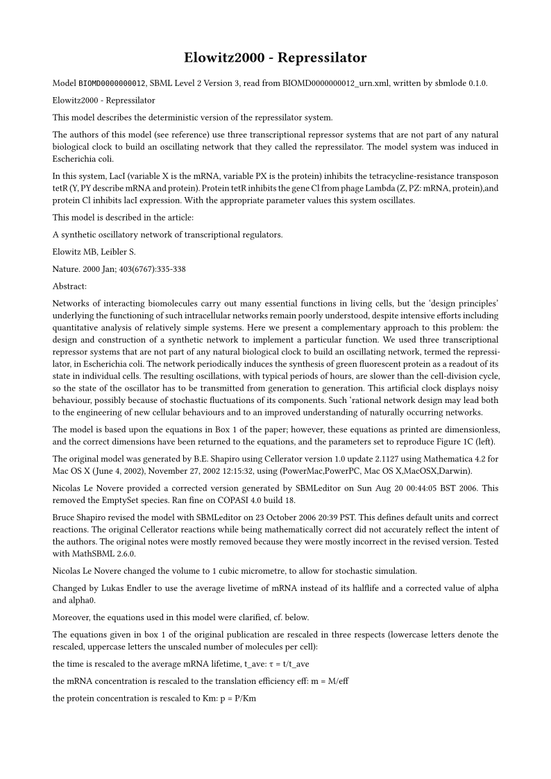
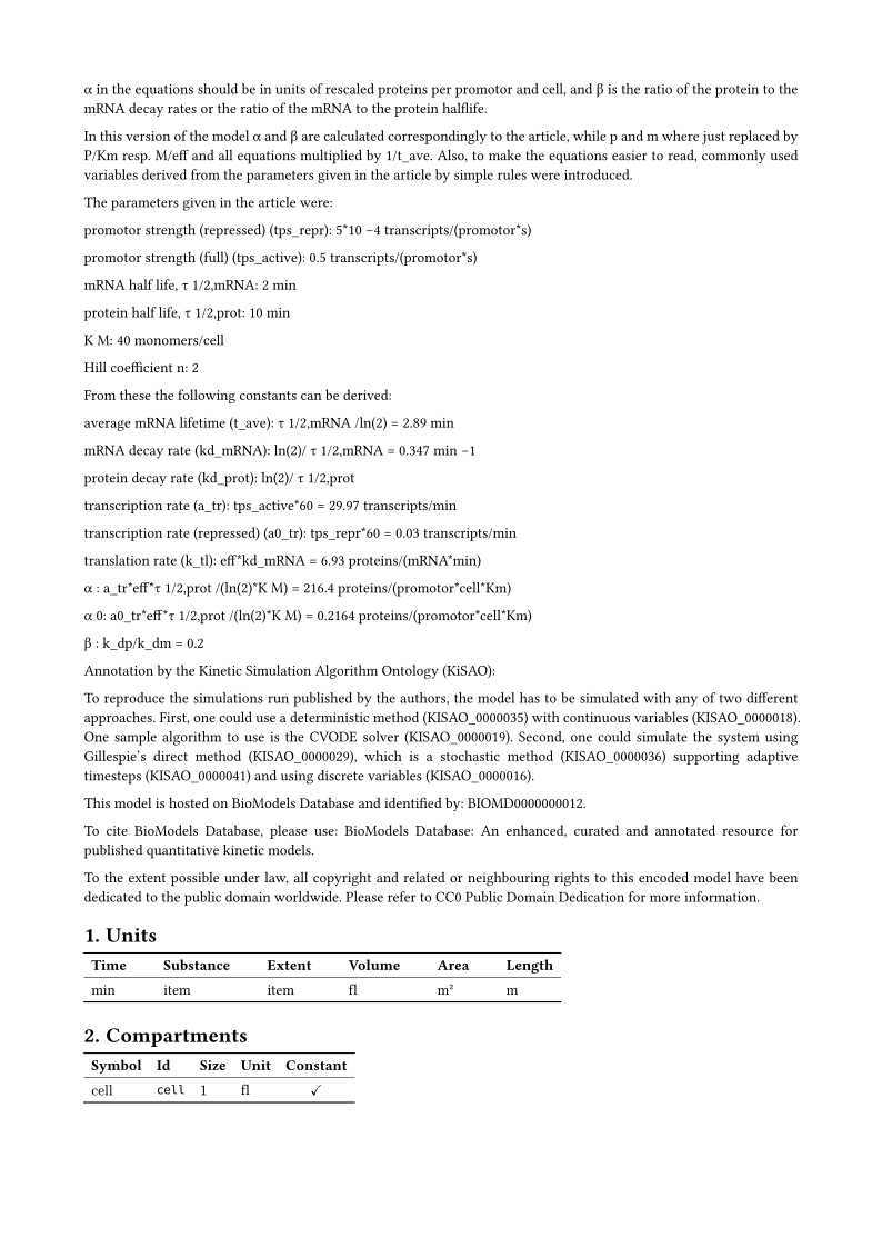
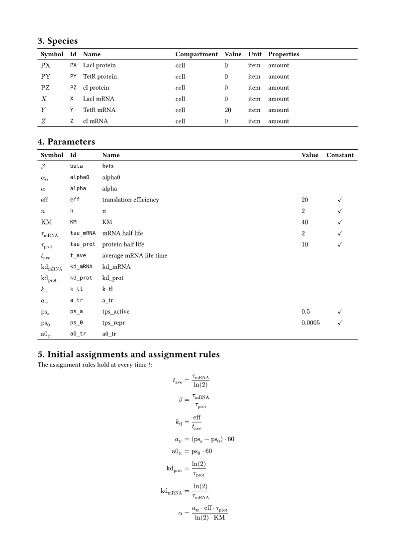
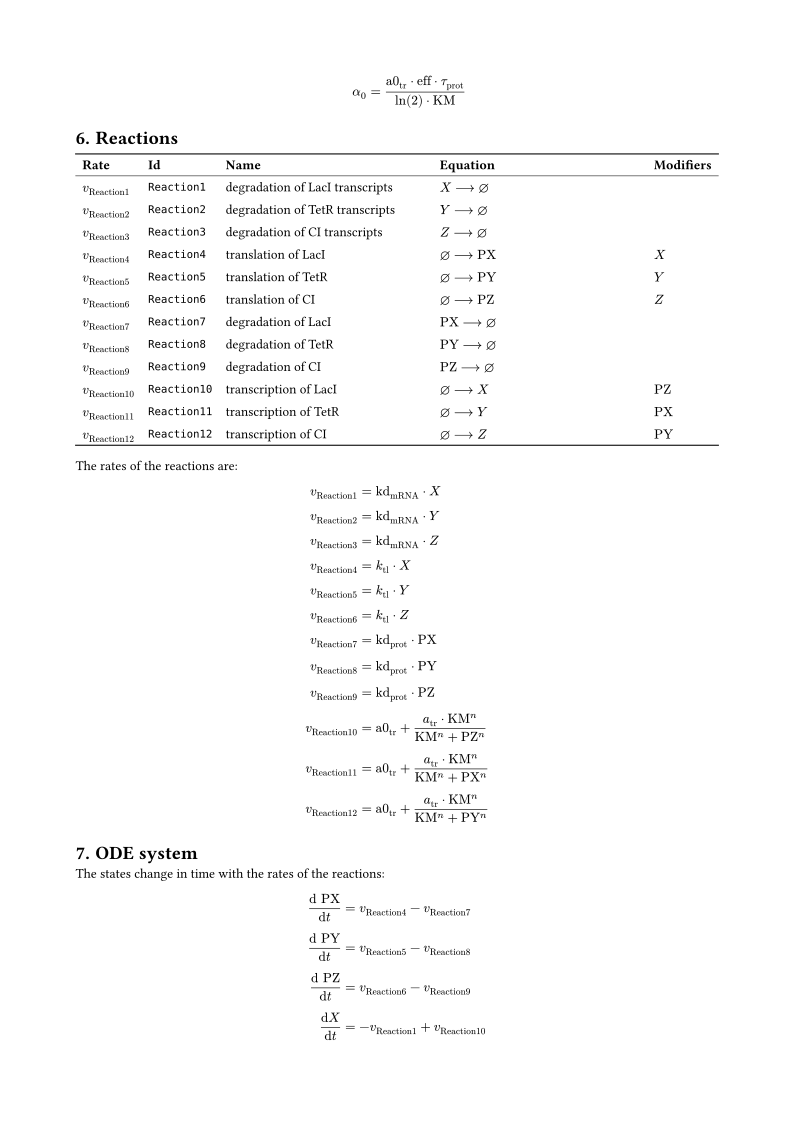
repressilator.typ, the typst source of the repressilator
#set document(title: [Elowitz2000 - Repressilator])
#set page(margin: 2cm)
#set text(size: 10pt)
#set par(justify: true)
#set heading(numbering: "1.")
// the equations of a section are one block, which breaks across pages
#show math.equation.where(block: true): set block(breakable: true)
#show math.equation.where(block: true): set par(leading: 0.9em)

#align(center, text(size: 16pt, weight: "bold")[Elowitz2000 - Repressilator])

Model `BIOMD0000000012`, SBML Level 2 Version 3, read from BIOMD0000000012\_urn.xml, written by sbmlode 0.1.0.

Elowitz2000 - Repressilator

This model describes the deterministic version of the repressilator system.

The authors of this model (see reference) use three transcriptional repressor systems that are not part of any natural biological clock to build an oscillating network that they called the repressilator. The model system was induced in Escherichia coli.

In this system, LacI (variable X is the mRNA, variable PX is the protein) inhibits the tetracycline-resistance transposon tetR (Y, PY describe mRNA and protein). Protein tetR inhibits the gene Cl from phage Lambda (Z, PZ: mRNA, protein),and protein Cl inhibits lacI expression. With the appropriate parameter values this system oscillates.

This model is described in the article:

A synthetic oscillatory network of transcriptional regulators.

Elowitz MB, Leibler S.

Nature. 2000 Jan; 403(6767):335-338

Abstract:

Networks of interacting biomolecules carry out many essential functions in living cells, but the 'design principles' underlying the functioning of such intracellular networks remain poorly understood, despite intensive efforts including quantitative analysis of relatively simple systems. Here we present a complementary approach to this problem: the design and construction of a synthetic network to implement a particular function. We used three transcriptional repressor systems that are not part of any natural biological clock to build an oscillating network, termed the repressilator, in Escherichia coli. The network periodically induces the synthesis of green fluorescent protein as a readout of its state in individual cells. The resulting oscillations, with typical periods of hours, are slower than the cell-division cycle, so the state of the oscillator has to be transmitted from generation to generation. This artificial clock displays noisy behaviour, possibly because of stochastic fluctuations of its components. Such 'rational network design may lead both to the engineering of new cellular behaviours and to an improved understanding of naturally occurring networks.

The model is based upon the equations in Box 1 of the paper; however, these equations as printed are dimensionless, and the correct dimensions have been returned to the equations, and the parameters set to reproduce Figure 1C (left).

The original model was generated by B.E. Shapiro using Cellerator version 1.0 update 2.1127 using Mathematica 4.2 for Mac OS X (June 4, 2002), November 27, 2002 12:15:32, using (PowerMac,PowerPC, Mac OS X,MacOSX,Darwin).

Nicolas Le Novere provided a corrected version generated by SBMLeditor on Sun Aug 20 00:44:05 BST 2006. This removed the EmptySet species. Ran fine on COPASI 4.0 build 18.

Bruce Shapiro revised the model with SBMLeditor on 23 October 2006 20:39 PST. This defines default units and correct reactions. The original Cellerator reactions while being mathematically correct did not accurately reflect the intent of the authors. The original notes were mostly removed because they were mostly incorrect in the revised version. Tested with MathSBML 2.6.0.

Nicolas Le Novere changed the volume to 1 cubic micrometre, to allow for stochastic simulation.

Changed by Lukas Endler to use the average livetime of mRNA instead of its halflife and a corrected value of alpha and alpha0.

Moreover, the equations used in this model were clarified, cf. below.

The equations given in box 1 of the original publication are rescaled in three respects (lowercase letters denote the rescaled, uppercase letters the unscaled number of molecules per cell):

the time is rescaled to the average mRNA lifetime, t\_ave: τ = t/t\_ave

the mRNA concentration is rescaled to the translation efficiency eff: m = M/eff

the protein concentration is rescaled to Km: p = P/Km

α in the equations should be in units of rescaled proteins per promotor and cell, and β is the ratio of the protein to the mRNA decay rates or the ratio of the mRNA to the protein halflife.

In this version of the model α and β are calculated correspondingly to the article, while p and m where just replaced by P/Km resp. M/eff and all equations multiplied by 1/t\_ave. Also, to make the equations easier to read, commonly used variables derived from the parameters given in the article by simple rules were introduced.

The parameters given in the article were:

promotor strength (repressed) (tps\_repr): 5\*10 -4 transcripts/(promotor\*s)

promotor strength (full) (tps\_active): 0.5 transcripts/(promotor\*s)

mRNA half life, τ 1/2,mRNA: 2 min

protein half life, τ 1/2,prot: 10 min

K M: 40 monomers/cell

Hill coefficient n: 2

From these the following constants can be derived:

average mRNA lifetime (t\_ave): τ 1/2,mRNA /ln(2) = 2.89 min

mRNA decay rate (kd\_mRNA): ln(2)/ τ 1/2,mRNA = 0.347 min -1

protein decay rate (kd\_prot): ln(2)/ τ 1/2,prot

transcription rate (a\_tr): tps\_active\*60 = 29.97 transcripts/min

transcription rate (repressed) (a0\_tr): tps\_repr\*60 = 0.03 transcripts/min

translation rate (k\_tl): eff\*kd\_mRNA = 6.93 proteins/(mRNA\*min)

α : a\_tr\*eff\*τ 1/2,prot /(ln(2)\*K M) = 216.4 proteins/(promotor\*cell\*Km)

α 0: a0\_tr\*eff\*τ 1/2,prot /(ln(2)\*K M) = 0.2164 proteins/(promotor\*cell\*Km)

β : k\_dp/k\_dm = 0.2

Annotation by the Kinetic Simulation Algorithm Ontology (KiSAO):

To reproduce the simulations run published by the authors, the model has to be simulated with any of two different approaches. First, one could use a deterministic method (KISAO\_0000035) with continuous variables (KISAO\_0000018). One sample algorithm to use is the CVODE solver (KISAO\_0000019). Second, one could simulate the system using Gillespie's direct method (KISAO\_0000029), which is a stochastic method (KISAO\_0000036) supporting adaptive timesteps (KISAO\_0000041) and using discrete variables (KISAO\_0000016).

This model is hosted on BioModels Database and identified by: BIOMD0000000012.

To cite BioModels Database, please use: BioModels Database: An enhanced, curated and annotated resource for published quantitative kinetic models.

To the extent possible under law, all copyright and related or neighbouring rights to this encoded model have been dedicated to the public domain worldwide. Please refer to CC0 Public Domain Dedication for more information.

= Units

#table(
  columns: 6,
  stroke: none,
  column-gutter: 1.5em,
  table.hline(stroke: 0.8pt),
  table.header([*Time*], [*Substance*], [*Extent*], [*Volume*], [*Area*], [*Length*]),
  table.hline(stroke: 0.4pt),
  [min], [item], [item], [#text(ligatures: false)[fl]], [m#super[2]], [m],
  table.hline(stroke: 0.8pt),
)

= Compartments

#table(
  columns: (auto, auto, auto, auto, auto),
  stroke: none,
  align: (left, left, left, left, center),
  table.hline(stroke: 0.8pt),
  table.header([*Symbol*], [*Id*], [*Size*], [*Unit*], [*Constant*]),
  table.hline(stroke: 0.4pt),
  [$upright("cell")$], [`cell`], [$1$], [#text(ligatures: false)[fl]], [#sym.checkmark],
  table.hline(stroke: 0.8pt),
)

= Species

#table(
  columns: (auto, auto, 1fr, auto, auto, auto, 1fr),
  stroke: none,
  align: (left, left, left, left, left, left, left),
  table.hline(stroke: 0.8pt),
  table.header([*Symbol*], [*Id*], [*Name*], [*Compartment*], [*Value*], [*Unit*], [*Properties*]),
  table.hline(stroke: 0.4pt),
  [$upright("PX")$], [`PX`], [LacI protein], [$upright("cell")$], [$0$], [item], [amount],
  [$upright("PY")$], [`PY`], [TetR protein], [$upright("cell")$], [$0$], [item], [amount],
  [$upright("PZ")$], [`PZ`], [cI protein], [$upright("cell")$], [$0$], [item], [amount],
  [$X$], [`X`], [LacI mRNA], [$upright("cell")$], [$0$], [item], [amount],
  [$Y$], [`Y`], [TetR mRNA], [$upright("cell")$], [$20$], [item], [amount],
  [$Z$], [`Z`], [cI mRNA], [$upright("cell")$], [$0$], [item], [amount],
  table.hline(stroke: 0.8pt),
)

= Parameters

#table(
  columns: (auto, auto, 1fr, auto, auto),
  stroke: none,
  align: (left, left, left, left, center),
  table.hline(stroke: 0.8pt),
  table.header([*Symbol*], [*Id*], [*Name*], [*Value*], [*Constant*]),
  table.hline(stroke: 0.4pt),
  [$beta$], [`beta`], [beta], [], [],
  [$alpha_(0)$], [`alpha0`], [alpha0], [], [],
  [$alpha$], [`alpha`], [alpha], [], [],
  [$upright("eff")$], [`eff`], [translation efficiency], [$20$], [#sym.checkmark],
  [$n$], [`n`], [n], [$2$], [#sym.checkmark],
  [$upright("KM")$], [`KM`], [KM], [$40$], [#sym.checkmark],
  [$tau_("mRNA")$], [`tau_mRNA`], [mRNA half life], [$2$], [#sym.checkmark],
  [$tau_("prot")$], [`tau_prot`], [protein half life], [$10$], [#sym.checkmark],
  [$t_("ave")$], [`t_ave`], [average mRNA life time], [], [],
  [$upright("kd")_("mRNA")$], [`kd_mRNA`], [kd\_mRNA], [], [],
  [$upright("kd")_("prot")$], [`kd_prot`], [kd\_prot], [], [],
  [$k_("tl")$], [`k_tl`], [k\_tl], [], [],
  [$a_("tr")$], [`a_tr`], [a\_tr], [], [],
  [$upright("ps")_("a")$], [`ps_a`], [tps\_active], [$0.5$], [#sym.checkmark],
  [$upright("ps")_(0)$], [`ps_0`], [tps\_repr], [$0.0005$], [#sym.checkmark],
  [$upright("a0")_("tr")$], [`a0_tr`], [a0\_tr], [], [],
  table.hline(stroke: 0.8pt),
)

= Initial assignments and assignment rules

The assignment rules hold at every time $t$:

$ t_("ave") &= (tau_("mRNA"))/(ln(2)) \
  beta &= (tau_("mRNA"))/(tau_("prot")) \
  k_("tl") &= (upright("eff"))/(t_("ave")) \
  a_("tr") &= (upright("ps")_("a") - upright("ps")_(0)) dot 60 \
  upright("a0")_("tr") &= upright("ps")_(0) dot 60 \
  upright("kd")_("prot") &= (ln(2))/(tau_("prot")) \
  upright("kd")_("mRNA") &= (ln(2))/(tau_("mRNA")) \
  alpha &= (a_("tr") dot upright("eff") dot tau_("prot"))/(ln(2) dot upright("KM")) \
  alpha_(0) &= (upright("a0")_("tr") dot upright("eff") dot tau_("prot"))/(ln(2) dot upright("KM")) $

= Reactions

#table(
  columns: (auto, auto, 1fr, 1fr, auto),
  stroke: none,
  align: (left, left, left, left, left),
  table.hline(stroke: 0.8pt),
  table.header([*Rate*], [*Id*], [*Name*], [*Equation*], [*Modifiers*]),
  table.hline(stroke: 0.4pt),
  [$v_("Reaction1")$], [`Reaction1`], [degradation of LacI transcripts], [$X --> emptyset$], [],
  [$v_("Reaction2")$], [`Reaction2`], [degradation of TetR transcripts], [$Y --> emptyset$], [],
  [$v_("Reaction3")$], [`Reaction3`], [degradation of CI transcripts], [$Z --> emptyset$], [],
  [$v_("Reaction4")$], [`Reaction4`], [translation of LacI], [$emptyset --> upright("PX")$], [$X$],
  [$v_("Reaction5")$], [`Reaction5`], [translation of TetR], [$emptyset --> upright("PY")$], [$Y$],
  [$v_("Reaction6")$], [`Reaction6`], [translation of CI], [$emptyset --> upright("PZ")$], [$Z$],
  [$v_("Reaction7")$], [`Reaction7`], [degradation of LacI], [$upright("PX") --> emptyset$], [],
  [$v_("Reaction8")$], [`Reaction8`], [degradation of TetR], [$upright("PY") --> emptyset$], [],
  [$v_("Reaction9")$], [`Reaction9`], [degradation of CI], [$upright("PZ") --> emptyset$], [],
  [$v_("Reaction10")$], [`Reaction10`], [transcription of LacI], [$emptyset --> X$], [$upright("PZ")$],
  [$v_("Reaction11")$], [`Reaction11`], [transcription of TetR], [$emptyset --> Y$], [$upright("PX")$],
  [$v_("Reaction12")$], [`Reaction12`], [transcription of CI], [$emptyset --> Z$], [$upright("PY")$],
  table.hline(stroke: 0.8pt),
)

The rates of the reactions are:

$ v_("Reaction1") &= upright("kd")_("mRNA") dot X \
  v_("Reaction2") &= upright("kd")_("mRNA") dot Y \
  v_("Reaction3") &= upright("kd")_("mRNA") dot Z \
  v_("Reaction4") &= k_("tl") dot X \
  v_("Reaction5") &= k_("tl") dot Y \
  v_("Reaction6") &= k_("tl") dot Z \
  v_("Reaction7") &= upright("kd")_("prot") dot upright("PX") \
  v_("Reaction8") &= upright("kd")_("prot") dot upright("PY") \
  v_("Reaction9") &= upright("kd")_("prot") dot upright("PZ") \
  v_("Reaction10") &= upright("a0")_("tr") + (a_("tr") dot upright("KM")^(n))/(upright("KM")^(n) + upright("PZ")^(n)) \
  v_("Reaction11") &= upright("a0")_("tr") + (a_("tr") dot upright("KM")^(n))/(upright("KM")^(n) + upright("PX")^(n)) \
  v_("Reaction12") &= upright("a0")_("tr") + (a_("tr") dot upright("KM")^(n))/(upright("KM")^(n) + upright("PY")^(n)) $

= ODE system

The states change in time with the rates of the reactions:

$ (dif upright("PX"))/(dif t) &= v_("Reaction4") - v_("Reaction7") \
  (dif upright("PY"))/(dif t) &= v_("Reaction5") - v_("Reaction8") \
  (dif upright("PZ"))/(dif t) &= v_("Reaction6") - v_("Reaction9") \
  (dif X)/(dif t) &= -v_("Reaction1") + v_("Reaction10") \
  (dif Y)/(dif t) &= -v_("Reaction2") + v_("Reaction11") \
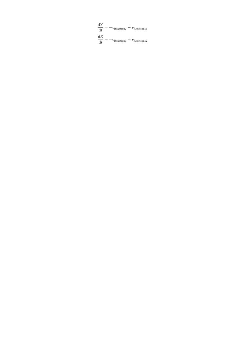
  (dif Z)/(dif t) &= -v_("Reaction3") + v_("Reaction12") $
LaTeX
The LaTeX document is an article with amsmath, amssymb, booktabs, xltabular, parskip and hyperref, which compiles with pdfLaTeX, XeLaTeX, LuaLaTeX or tectonic:
The fragment of standalone=False is the body of the document, whose title is a \section, and is included with \input{repressilator.tex} into a document which loads amsmath, amssymb, booktabs and xltabular; a comment at its top names them.
repressilator.tex, the LaTeX source of the repressilator
\documentclass{article}
\usepackage{iftex}
\ifPDFTeX
  \usepackage[T1]{fontenc}
  \usepackage{lmodern}
\else
  \usepackage{fontspec}
\fi
\usepackage{amsmath, amssymb, booktabs, xltabular, parskip, hyperref}
\usepackage[margin=2cm]{geometry}
% the equations of a section are one alignment, which breaks across pages
\allowdisplaybreaks
\setlength{\jot}{1.5ex}
\renewcommand{\arraystretch}{1.15}

\begin{document}

{\centering\LARGE\bfseries Elowitz2000 - Repressilator\par}
\bigskip

Model \texttt{BIOMD0000000012}, SBML Level 2 Version 3, read from BIOMD0000000012\_\allowbreak{}urn.xml, written by sbmlode 0.1.0.

Elowitz2000 - Repressilator

This model describes the deterministic version of the repressilator system.

The authors of this model (see reference) use three transcriptional repressor systems that are not part of any natural biological clock to build an oscillating network that they called the repressilator. The model system was induced in Escherichia coli.

In this system, LacI (variable X is the mRNA, variable PX is the protein) inhibits the tetracycline-resistance transposon tetR (Y, PY describe mRNA and protein). Protein tetR inhibits the gene Cl from phage Lambda (Z, PZ: mRNA, protein),and protein Cl inhibits lacI expression. With the appropriate parameter values this system oscillates.

This model is described in the article:

A synthetic oscillatory network of transcriptional regulators.

Elowitz MB, Leibler S.

Nature. 2000 Jan; 403(6767):335-338

Abstract:

Networks of interacting biomolecules carry out many essential functions in living cells, but the 'design principles' underlying the functioning of such intracellular networks remain poorly understood, despite intensive efforts including quantitative analysis of relatively simple systems. Here we present a complementary approach to this problem: the design and construction of a synthetic network to implement a particular function. We used three transcriptional repressor systems that are not part of any natural biological clock to build an oscillating network, termed the repressilator, in Escherichia coli. The network periodically induces the synthesis of green fluorescent protein as a readout of its state in individual cells. The resulting oscillations, with typical periods of hours, are slower than the cell-division cycle, so the state of the oscillator has to be transmitted from generation to generation. This artificial clock displays noisy behaviour, possibly because of stochastic fluctuations of its components. Such 'rational network design may lead both to the engineering of new cellular behaviours and to an improved understanding of naturally occurring networks.

The model is based upon the equations in Box 1 of the paper; however, these equations as printed are dimensionless, and the correct dimensions have been returned to the equations, and the parameters set to reproduce Figure 1C (left).

The original model was generated by B.E. Shapiro using Cellerator version 1.0 update 2.1127 using Mathematica 4.2 for Mac OS X (June 4, 2002), November 27, 2002 12:15:32, using (PowerMac,PowerPC, Mac OS X,MacOSX,Darwin).

Nicolas Le Novere provided a corrected version generated by SBMLeditor on Sun Aug 20 00:44:05 BST 2006. This removed the EmptySet species. Ran fine on COPASI 4.0 build 18.

Bruce Shapiro revised the model with SBMLeditor on 23 October 2006 20:39 PST. This defines default units and correct reactions. The original Cellerator reactions while being mathematically correct did not accurately reflect the intent of the authors. The original notes were mostly removed because they were mostly incorrect in the revised version. Tested with MathSBML 2.6.0.

Nicolas Le Novere changed the volume to 1 cubic micrometre, to allow for stochastic simulation.

Changed by Lukas Endler to use the average livetime of mRNA instead of its halflife and a corrected value of alpha and alpha0.

Moreover, the equations used in this model were clarified, cf. below.

The equations given in box 1 of the original publication are rescaled in three respects (lowercase letters denote the rescaled, uppercase letters the unscaled number of molecules per cell):

the time is rescaled to the average mRNA lifetime, t\_ave: \ensuremath{\tau} = t/t\_ave

the mRNA concentration is rescaled to the translation efficiency eff: m = M/eff

the protein concentration is rescaled to Km: p = P/Km

\ensuremath{\alpha} in the equations should be in units of rescaled proteins per promotor and cell, and \ensuremath{\beta} is the ratio of the protein to the mRNA decay rates or the ratio of the mRNA to the protein halflife.

In this version of the model \ensuremath{\alpha} and \ensuremath{\beta} are calculated correspondingly to the article, while p and m where just replaced by P/Km resp. M/eff and all equations multiplied by 1/t\_ave. Also, to make the equations easier to read, commonly used variables derived from the parameters given in the article by simple rules were introduced.

The parameters given in the article were:

promotor strength (repressed) (tps\_repr): 5*10 -4 transcripts/(promotor*s)

promotor strength (full) (tps\_active): 0.5 transcripts/(promotor*s)

mRNA half life, \ensuremath{\tau} 1/2,mRNA: 2 min

protein half life, \ensuremath{\tau} 1/2,prot: 10 min

K M: 40 monomers/cell

Hill coefficient n: 2

From these the following constants can be derived:

average mRNA lifetime (t\_ave): \ensuremath{\tau} 1/2,mRNA /ln(2) = 2.89 min

mRNA decay rate (kd\_mRNA): ln(2)/ \ensuremath{\tau} 1/2,mRNA = 0.347 min -1

protein decay rate (kd\_prot): ln(2)/ \ensuremath{\tau} 1/2,prot

transcription rate (a\_tr): tps\_active*60 = 29.97 transcripts/min

transcription rate (repressed) (a0\_tr): tps\_repr*60 = 0.03 transcripts/min

translation rate (k\_tl): eff*kd\_mRNA = 6.93 proteins/(mRNA*min)

\ensuremath{\alpha} : a\_tr*eff*\ensuremath{\tau} 1/2,prot /(ln(2)*K M) = 216.4 proteins/(promotor*cell*Km)

\ensuremath{\alpha} 0: a0\_tr*eff*\ensuremath{\tau} 1/2,prot /(ln(2)*K M) = 0.2164 proteins/(promotor*cell*Km)

\ensuremath{\beta} : k\_dp/k\_dm = 0.2

Annotation by the Kinetic Simulation Algorithm Ontology (KiSAO):

To reproduce the simulations run published by the authors, the model has to be simulated with any of two different approaches. First, one could use a deterministic method (KISAO\_0000035) with continuous variables (KISAO\_0000018). One sample algorithm to use is the CVODE solver (KISAO\_0000019). Second, one could simulate the system using Gillespie's direct method (KISAO\_0000029), which is a stochastic method (KISAO\_0000036) supporting adaptive timesteps (KISAO\_0000041) and using discrete variables (KISAO\_0000016).

This model is hosted on BioModels Database and identified by: BIOMD0000000012.

To cite BioModels Database, please use: BioModels Database: An enhanced, curated and annotated resource for published quantitative kinetic models.

To the extent possible under law, all copyright and related or neighbouring rights to this encoded model have been dedicated to the public domain worldwide. Please refer to CC0 Public Domain Dedication for more information.

\section{Units}

\begin{tabular}{@{}llllll@{}}
  \toprule
  \textbf{Time} & \textbf{Substance} & \textbf{Extent} & \textbf{Volume} & \textbf{Area} & \textbf{Length} \\
  \midrule
  min & item & item & f\kern0pt{}l & m\textsuperscript{2} & m \\
  \bottomrule
\end{tabular}

\section{Compartments}

\begin{longtable}[l]{@{}l l l l c@{}}
  \toprule
  \textbf{Symbol} & \textbf{Id} & \textbf{Size} & \textbf{Unit} & \textbf{Constant} \\
  \midrule
  \endhead
  \bottomrule
  \endfoot
  $\mathrm{cell}$ & \texttt{cell} & $1$ & f\kern0pt{}l & $\checkmark$ \\
\end{longtable}

\section{Species}

\begin{xltabular}{\linewidth}{@{}l l >{\raggedright\arraybackslash\hspace{0pt}}X l l l >{\raggedright\arraybackslash\hspace{0pt}}X@{}}
  \toprule
  \textbf{Symbol} & \textbf{Id} & \textbf{Name} & \textbf{Compartment} & \textbf{Value} & \textbf{Unit} & \textbf{Properties} \\
  \midrule
  \endhead
  \bottomrule
  \endfoot
  $\mathrm{PX}$ & \texttt{PX} & LacI protein & $\mathrm{cell}$ & $0$ & item & amount \\
  $\mathrm{PY}$ & \texttt{PY} & TetR protein & $\mathrm{cell}$ & $0$ & item & amount \\
  $\mathrm{PZ}$ & \texttt{PZ} & cI protein & $\mathrm{cell}$ & $0$ & item & amount \\
  $X$ & \texttt{X} & LacI mRNA & $\mathrm{cell}$ & $0$ & item & amount \\
  $Y$ & \texttt{Y} & TetR mRNA & $\mathrm{cell}$ & $20$ & item & amount \\
  $Z$ & \texttt{Z} & cI mRNA & $\mathrm{cell}$ & $0$ & item & amount \\
\end{xltabular}

\section{Parameters}

\begin{xltabular}{\linewidth}{@{}l l >{\raggedright\arraybackslash\hspace{0pt}}X l c@{}}
  \toprule
  \textbf{Symbol} & \textbf{Id} & \textbf{Name} & \textbf{Value} & \textbf{Constant} \\
  \midrule
  \endhead
  \bottomrule
  \endfoot
  $\beta$ & \texttt{beta} & beta &  &  \\
  $\alpha_{0}$ & \texttt{alpha0} & alpha0 &  &  \\
  $\alpha$ & \texttt{alpha} & alpha &  &  \\
  $\mathrm{eff}$ & \texttt{eff} & translation efficiency & $20$ & $\checkmark$ \\
  $n$ & \texttt{n} & n & $2$ & $\checkmark$ \\
  $\mathrm{KM}$ & \texttt{KM} & KM & $40$ & $\checkmark$ \\
  $\tau_{\mathrm{mRNA}}$ & \texttt{tau\_mRNA} & mRNA half life & $2$ & $\checkmark$ \\
  $\tau_{\mathrm{prot}}$ & \texttt{tau\_prot} & protein half life & $10$ & $\checkmark$ \\
  $t_{\mathrm{ave}}$ & \texttt{t\_ave} & average mRNA life time &  &  \\
  $\mathrm{kd}_{\mathrm{mRNA}}$ & \texttt{kd\_mRNA} & kd\_mRNA &  &  \\
  $\mathrm{kd}_{\mathrm{prot}}$ & \texttt{kd\_prot} & kd\_prot &  &  \\
  $k_{\mathrm{tl}}$ & \texttt{k\_tl} & k\_tl &  &  \\
  $a_{\mathrm{tr}}$ & \texttt{a\_tr} & a\_tr &  &  \\
  $\mathrm{ps}_{\mathrm{a}}$ & \texttt{ps\_a} & tps\_active & $0.5$ & $\checkmark$ \\
  $\mathrm{ps}_{0}$ & \texttt{ps\_0} & tps\_repr & $0.0005$ & $\checkmark$ \\
  $\mathrm{a0}_{\mathrm{tr}}$ & \texttt{a0\_tr} & a0\_tr &  &  \\
\end{xltabular}

\section{Initial assignments and assignment rules}

The assignment rules hold at every time $t$:
\begin{align*}
  t_{\mathrm{ave}} &= \frac{\tau_{\mathrm{mRNA}}}{\ln\mathopen{}\left(2\right)} \\
  \beta &= \frac{\tau_{\mathrm{mRNA}}}{\tau_{\mathrm{prot}}} \\
  k_{\mathrm{tl}} &= \frac{\mathrm{eff}}{t_{\mathrm{ave}}} \\
  a_{\mathrm{tr}} &= \mathopen{}\left(\mathrm{ps}_{\mathrm{a}} - \mathrm{ps}_{0}\right) \cdot 60 \\
  \mathrm{a0}_{\mathrm{tr}} &= \mathrm{ps}_{0} \cdot 60 \\
  \mathrm{kd}_{\mathrm{prot}} &= \frac{\ln\mathopen{}\left(2\right)}{\tau_{\mathrm{prot}}} \\
  \mathrm{kd}_{\mathrm{mRNA}} &= \frac{\ln\mathopen{}\left(2\right)}{\tau_{\mathrm{mRNA}}} \\
  \alpha &= \frac{a_{\mathrm{tr}} \cdot \mathrm{eff} \cdot \tau_{\mathrm{prot}}}{\ln\mathopen{}\left(2\right) \cdot \mathrm{KM}} \\
  \alpha_{0} &= \frac{\mathrm{a0}_{\mathrm{tr}} \cdot \mathrm{eff} \cdot \tau_{\mathrm{prot}}}{\ln\mathopen{}\left(2\right) \cdot \mathrm{KM}}
\end{align*}

\section{Reactions}

\begin{xltabular}{\linewidth}{@{}l l >{\raggedright\arraybackslash\hspace{0pt}}X >{\raggedright\arraybackslash\hspace{0pt}}X l@{}}
  \toprule
  \textbf{Rate} & \textbf{Id} & \textbf{Name} & \textbf{Equation} & \textbf{Modifiers} \\
  \midrule
  \endhead
  \bottomrule
  \endfoot
  $v_{\mathrm{Reaction1}}$ & \texttt{Reaction1} & degradation of LacI transcripts & $X \longrightarrow \varnothing$ &  \\
  $v_{\mathrm{Reaction2}}$ & \texttt{Reaction2} & degradation of TetR transcripts & $Y \longrightarrow \varnothing$ &  \\
  $v_{\mathrm{Reaction3}}$ & \texttt{Reaction3} & degradation of CI transcripts & $Z \longrightarrow \varnothing$ &  \\
  $v_{\mathrm{Reaction4}}$ & \texttt{Reaction4} & translation of LacI & $\varnothing \longrightarrow \mathrm{PX}$ & $X$ \\
  $v_{\mathrm{Reaction5}}$ & \texttt{Reaction5} & translation of TetR & $\varnothing \longrightarrow \mathrm{PY}$ & $Y$ \\
  $v_{\mathrm{Reaction6}}$ & \texttt{Reaction6} & translation of CI & $\varnothing \longrightarrow \mathrm{PZ}$ & $Z$ \\
  $v_{\mathrm{Reaction7}}$ & \texttt{Reaction7} & degradation of LacI & $\mathrm{PX} \longrightarrow \varnothing$ &  \\
  $v_{\mathrm{Reaction8}}$ & \texttt{Reaction8} & degradation of TetR & $\mathrm{PY} \longrightarrow \varnothing$ &  \\
  $v_{\mathrm{Reaction9}}$ & \texttt{Reaction9} & degradation of CI & $\mathrm{PZ} \longrightarrow \varnothing$ &  \\
  $v_{\mathrm{Reaction10}}$ & \texttt{Reaction10} & transcription of LacI & $\varnothing \longrightarrow X$ & $\mathrm{PZ}$ \\
  $v_{\mathrm{Reaction11}}$ & \texttt{Reaction11} & transcription of TetR & $\varnothing \longrightarrow Y$ & $\mathrm{PX}$ \\
  $v_{\mathrm{Reaction12}}$ & \texttt{Reaction12} & transcription of CI & $\varnothing \longrightarrow Z$ & $\mathrm{PY}$ \\
\end{xltabular}

The rates of the reactions are:
\begin{align*}
  v_{\mathrm{Reaction1}} &= \mathrm{kd}_{\mathrm{mRNA}} \cdot X \\
  v_{\mathrm{Reaction2}} &= \mathrm{kd}_{\mathrm{mRNA}} \cdot Y \\
  v_{\mathrm{Reaction3}} &= \mathrm{kd}_{\mathrm{mRNA}} \cdot Z \\
  v_{\mathrm{Reaction4}} &= k_{\mathrm{tl}} \cdot X \\
  v_{\mathrm{Reaction5}} &= k_{\mathrm{tl}} \cdot Y \\
  v_{\mathrm{Reaction6}} &= k_{\mathrm{tl}} \cdot Z \\
  v_{\mathrm{Reaction7}} &= \mathrm{kd}_{\mathrm{prot}} \cdot \mathrm{PX} \\
  v_{\mathrm{Reaction8}} &= \mathrm{kd}_{\mathrm{prot}} \cdot \mathrm{PY} \\
  v_{\mathrm{Reaction9}} &= \mathrm{kd}_{\mathrm{prot}} \cdot \mathrm{PZ} \\
  v_{\mathrm{Reaction10}} &= \mathrm{a0}_{\mathrm{tr}} + \frac{a_{\mathrm{tr}} \cdot \mathrm{KM}^{n}}{\mathrm{KM}^{n} + \mathrm{PZ}^{n}} \\
  v_{\mathrm{Reaction11}} &= \mathrm{a0}_{\mathrm{tr}} + \frac{a_{\mathrm{tr}} \cdot \mathrm{KM}^{n}}{\mathrm{KM}^{n} + \mathrm{PX}^{n}} \\
  v_{\mathrm{Reaction12}} &= \mathrm{a0}_{\mathrm{tr}} + \frac{a_{\mathrm{tr}} \cdot \mathrm{KM}^{n}}{\mathrm{KM}^{n} + \mathrm{PY}^{n}}
\end{align*}

\section{ODE system}

The states change in time with the rates of the reactions:
\begin{align*}
  \frac{\mathrm{d} \,\mathrm{PX}}{\mathrm{d} t} &= v_{\mathrm{Reaction4}} - v_{\mathrm{Reaction7}} \\
  \frac{\mathrm{d} \,\mathrm{PY}}{\mathrm{d} t} &= v_{\mathrm{Reaction5}} - v_{\mathrm{Reaction8}} \\
  \frac{\mathrm{d} \,\mathrm{PZ}}{\mathrm{d} t} &= v_{\mathrm{Reaction6}} - v_{\mathrm{Reaction9}} \\
  \frac{\mathrm{d} X}{\mathrm{d} t} &= -v_{\mathrm{Reaction1}} + v_{\mathrm{Reaction10}} \\
  \frac{\mathrm{d} Y}{\mathrm{d} t} &= -v_{\mathrm{Reaction2}} + v_{\mathrm{Reaction11}} \\
  \frac{\mathrm{d} Z}{\mathrm{d} t} &= -v_{\mathrm{Reaction3}} + v_{\mathrm{Reaction12}}
\end{align*}

\end{document}
Markdown
The markdown is GitHub flavored markdown, with tables and the math as LaTeX in $...$ and $$...$$, which GitHub renders, as does this documentation with MathJax (pymdownx.arithmatex). It is the markdown which create_model(..., create_markdown=True) writes next to the SBML file, see Model creation of sbmlutils.
repressilator.md, the markdown source of the repressilator
# Elowitz2000 - Repressilator

Model `BIOMD0000000012`, SBML Level 2 Version 3, read from BIOMD0000000012\_urn.xml, written by sbmlode 0.1.0.

Elowitz2000 - Repressilator

This model describes the deterministic version of the repressilator system.

The authors of this model (see reference) use three transcriptional repressor systems that are not part of any natural biological clock to build an oscillating network that they called the repressilator. The model system was induced in Escherichia coli.

In this system, LacI (variable X is the mRNA, variable PX is the protein) inhibits the tetracycline-resistance transposon tetR (Y, PY describe mRNA and protein). Protein tetR inhibits the gene Cl from phage Lambda (Z, PZ: mRNA, protein),and protein Cl inhibits lacI expression. With the appropriate parameter values this system oscillates.

This model is described in the article:

A synthetic oscillatory network of transcriptional regulators.

Elowitz MB, Leibler S.

Nature. 2000 Jan; 403(6767):335-338

Abstract:

Networks of interacting biomolecules carry out many essential functions in living cells, but the 'design principles' underlying the functioning of such intracellular networks remain poorly understood, despite intensive efforts including quantitative analysis of relatively simple systems. Here we present a complementary approach to this problem: the design and construction of a synthetic network to implement a particular function. We used three transcriptional repressor systems that are not part of any natural biological clock to build an oscillating network, termed the repressilator, in Escherichia coli. The network periodically induces the synthesis of green fluorescent protein as a readout of its state in individual cells. The resulting oscillations, with typical periods of hours, are slower than the cell-division cycle, so the state of the oscillator has to be transmitted from generation to generation. This artificial clock displays noisy behaviour, possibly because of stochastic fluctuations of its components. Such 'rational network design may lead both to the engineering of new cellular behaviours and to an improved understanding of naturally occurring networks.

The model is based upon the equations in Box 1 of the paper; however, these equations as printed are dimensionless, and the correct dimensions have been returned to the equations, and the parameters set to reproduce Figure 1C (left).

The original model was generated by B.E. Shapiro using Cellerator version 1.0 update 2.1127 using Mathematica 4.2 for Mac OS X (June 4, 2002), November 27, 2002 12:15:32, using (PowerMac,PowerPC, Mac OS X,MacOSX,Darwin).

Nicolas Le Novere provided a corrected version generated by SBMLeditor on Sun Aug 20 00:44:05 BST 2006. This removed the EmptySet species. Ran fine on COPASI 4.0 build 18.

Bruce Shapiro revised the model with SBMLeditor on 23 October 2006 20:39 PST. This defines default units and correct reactions. The original Cellerator reactions while being mathematically correct did not accurately reflect the intent of the authors. The original notes were mostly removed because they were mostly incorrect in the revised version. Tested with MathSBML 2.6.0.

Nicolas Le Novere changed the volume to 1 cubic micrometre, to allow for stochastic simulation.

Changed by Lukas Endler to use the average livetime of mRNA instead of its halflife and a corrected value of alpha and alpha0.

Moreover, the equations used in this model were clarified, cf. below.

The equations given in box 1 of the original publication are rescaled in three respects (lowercase letters denote the rescaled, uppercase letters the unscaled number of molecules per cell):

the time is rescaled to the average mRNA lifetime, t\_ave: τ = t/t\_ave

the mRNA concentration is rescaled to the translation efficiency eff: m = M/eff

the protein concentration is rescaled to Km: p = P/Km

α in the equations should be in units of rescaled proteins per promotor and cell, and β is the ratio of the protein to the mRNA decay rates or the ratio of the mRNA to the protein halflife.

In this version of the model α and β are calculated correspondingly to the article, while p and m where just replaced by P/Km resp. M/eff and all equations multiplied by 1/t\_ave. Also, to make the equations easier to read, commonly used variables derived from the parameters given in the article by simple rules were introduced.

The parameters given in the article were:

promotor strength (repressed) (tps\_repr): 5\*10 -4 transcripts/(promotor\*s)

promotor strength (full) (tps\_active): 0.5 transcripts/(promotor\*s)

mRNA half life, τ 1/2,mRNA: 2 min

protein half life, τ 1/2,prot: 10 min

K M: 40 monomers/cell

Hill coefficient n: 2

From these the following constants can be derived:

average mRNA lifetime (t\_ave): τ 1/2,mRNA /ln(2) = 2.89 min

mRNA decay rate (kd\_mRNA): ln(2)/ τ 1/2,mRNA = 0.347 min -1

protein decay rate (kd\_prot): ln(2)/ τ 1/2,prot

transcription rate (a\_tr): tps\_active\*60 = 29.97 transcripts/min

transcription rate (repressed) (a0\_tr): tps\_repr\*60 = 0.03 transcripts/min

translation rate (k\_tl): eff\*kd\_mRNA = 6.93 proteins/(mRNA\*min)

α : a\_tr\*eff\*τ 1/2,prot /(ln(2)\*K M) = 216.4 proteins/(promotor\*cell\*Km)

α 0: a0\_tr\*eff\*τ 1/2,prot /(ln(2)\*K M) = 0.2164 proteins/(promotor\*cell\*Km)

β : k\_dp/k\_dm = 0.2

Annotation by the Kinetic Simulation Algorithm Ontology (KiSAO):

To reproduce the simulations run published by the authors, the model has to be simulated with any of two different approaches. First, one could use a deterministic method (KISAO\_0000035) with continuous variables (KISAO\_0000018). One sample algorithm to use is the CVODE solver (KISAO\_0000019). Second, one could simulate the system using Gillespie's direct method (KISAO\_0000029), which is a stochastic method (KISAO\_0000036) supporting adaptive timesteps (KISAO\_0000041) and using discrete variables (KISAO\_0000016).

This model is hosted on BioModels Database and identified by: BIOMD0000000012.

To cite BioModels Database, please use: BioModels Database: An enhanced, curated and annotated resource for published quantitative kinetic models.

To the extent possible under law, all copyright and related or neighbouring rights to this encoded model have been dedicated to the public domain worldwide. Please refer to CC0 Public Domain Dedication for more information.

## Units

| Time | Substance | Extent | Volume | Area | Length |
| --- | --- | --- | --- | --- | --- |
| min | item | item | fl | m<sup>2</sup> | m |

## Compartments

| Symbol | Id | Size | Unit | Constant |
| --- | --- | --- | --- | :---: |
| $\mathrm{cell}$ | `cell` | $1$ | fl | ✓ |

## Species

| Symbol | Id | Name | Compartment | Value | Unit | Properties |
| --- | --- | --- | --- | --- | --- | --- |
| $\mathrm{PX}$ | `PX` | LacI protein | $\mathrm{cell}$ | $0$ | item | amount |
| $\mathrm{PY}$ | `PY` | TetR protein | $\mathrm{cell}$ | $0$ | item | amount |
| $\mathrm{PZ}$ | `PZ` | cI protein | $\mathrm{cell}$ | $0$ | item | amount |
| $X$ | `X` | LacI mRNA | $\mathrm{cell}$ | $0$ | item | amount |
| $Y$ | `Y` | TetR mRNA | $\mathrm{cell}$ | $20$ | item | amount |
| $Z$ | `Z` | cI mRNA | $\mathrm{cell}$ | $0$ | item | amount |

## Parameters

| Symbol | Id | Name | Value | Constant |
| --- | --- | --- | --- | :---: |
| $\beta$ | `beta` | beta |  |  |
| $\alpha_{0}$ | `alpha0` | alpha0 |  |  |
| $\alpha$ | `alpha` | alpha |  |  |
| $\mathrm{eff}$ | `eff` | translation efficiency | $20$ | ✓ |
| $n$ | `n` | n | $2$ | ✓ |
| $\mathrm{KM}$ | `KM` | KM | $40$ | ✓ |
| $\tau_{\mathrm{mRNA}}$ | `tau_mRNA` | mRNA half life | $2$ | ✓ |
| $\tau_{\mathrm{prot}}$ | `tau_prot` | protein half life | $10$ | ✓ |
| $t_{\mathrm{ave}}$ | `t_ave` | average mRNA life time |  |  |
| $\mathrm{kd}_{\mathrm{mRNA}}$ | `kd_mRNA` | kd\_mRNA |  |  |
| $\mathrm{kd}_{\mathrm{prot}}$ | `kd_prot` | kd\_prot |  |  |
| $k_{\mathrm{tl}}$ | `k_tl` | k\_tl |  |  |
| $a_{\mathrm{tr}}$ | `a_tr` | a\_tr |  |  |
| $\mathrm{ps}_{\mathrm{a}}$ | `ps_a` | tps\_active | $0.5$ | ✓ |
| $\mathrm{ps}_{0}$ | `ps_0` | tps\_repr | $0.0005$ | ✓ |
| $\mathrm{a0}_{\mathrm{tr}}$ | `a0_tr` | a0\_tr |  |  |

## Initial assignments and assignment rules

The assignment rules hold at every time $t$:

$$
\begin{aligned}
t_{\mathrm{ave}} &= \frac{\tau_{\mathrm{mRNA}}}{\ln\mathopen{}\left(2\right)} \\[1ex]
\beta &= \frac{\tau_{\mathrm{mRNA}}}{\tau_{\mathrm{prot}}} \\[1ex]
k_{\mathrm{tl}} &= \frac{\mathrm{eff}}{t_{\mathrm{ave}}} \\[1ex]
a_{\mathrm{tr}} &= \mathopen{}\left(\mathrm{ps}_{\mathrm{a}} - \mathrm{ps}_{0}\right) \cdot 60 \\[1ex]
\mathrm{a0}_{\mathrm{tr}} &= \mathrm{ps}_{0} \cdot 60 \\[1ex]
\mathrm{kd}_{\mathrm{prot}} &= \frac{\ln\mathopen{}\left(2\right)}{\tau_{\mathrm{prot}}} \\[1ex]
\mathrm{kd}_{\mathrm{mRNA}} &= \frac{\ln\mathopen{}\left(2\right)}{\tau_{\mathrm{mRNA}}} \\[1ex]
\alpha &= \frac{a_{\mathrm{tr}} \cdot \mathrm{eff} \cdot \tau_{\mathrm{prot}}}{\ln\mathopen{}\left(2\right) \cdot \mathrm{KM}} \\[1ex]
\alpha_{0} &= \frac{\mathrm{a0}_{\mathrm{tr}} \cdot \mathrm{eff} \cdot \tau_{\mathrm{prot}}}{\ln\mathopen{}\left(2\right) \cdot \mathrm{KM}}
\end{aligned}
$$

## Reactions

| Rate | Id | Name | Equation | Modifiers |
| --- | --- | --- | --- | --- |
| $v_{\mathrm{Reaction1}}$ | `Reaction1` | degradation of LacI transcripts | $X \longrightarrow \varnothing$ |  |
| $v_{\mathrm{Reaction2}}$ | `Reaction2` | degradation of TetR transcripts | $Y \longrightarrow \varnothing$ |  |
| $v_{\mathrm{Reaction3}}$ | `Reaction3` | degradation of CI transcripts | $Z \longrightarrow \varnothing$ |  |
| $v_{\mathrm{Reaction4}}$ | `Reaction4` | translation of LacI | $\varnothing \longrightarrow \mathrm{PX}$ | $X$ |
| $v_{\mathrm{Reaction5}}$ | `Reaction5` | translation of TetR | $\varnothing \longrightarrow \mathrm{PY}$ | $Y$ |
| $v_{\mathrm{Reaction6}}$ | `Reaction6` | translation of CI | $\varnothing \longrightarrow \mathrm{PZ}$ | $Z$ |
| $v_{\mathrm{Reaction7}}$ | `Reaction7` | degradation of LacI | $\mathrm{PX} \longrightarrow \varnothing$ |  |
| $v_{\mathrm{Reaction8}}$ | `Reaction8` | degradation of TetR | $\mathrm{PY} \longrightarrow \varnothing$ |  |
| $v_{\mathrm{Reaction9}}$ | `Reaction9` | degradation of CI | $\mathrm{PZ} \longrightarrow \varnothing$ |  |
| $v_{\mathrm{Reaction10}}$ | `Reaction10` | transcription of LacI | $\varnothing \longrightarrow X$ | $\mathrm{PZ}$ |
| $v_{\mathrm{Reaction11}}$ | `Reaction11` | transcription of TetR | $\varnothing \longrightarrow Y$ | $\mathrm{PX}$ |
| $v_{\mathrm{Reaction12}}$ | `Reaction12` | transcription of CI | $\varnothing \longrightarrow Z$ | $\mathrm{PY}$ |

The rates of the reactions are:

$$
\begin{aligned}
v_{\mathrm{Reaction1}} &= \mathrm{kd}_{\mathrm{mRNA}} \cdot X \\[1ex]
v_{\mathrm{Reaction2}} &= \mathrm{kd}_{\mathrm{mRNA}} \cdot Y \\[1ex]
v_{\mathrm{Reaction3}} &= \mathrm{kd}_{\mathrm{mRNA}} \cdot Z \\[1ex]
v_{\mathrm{Reaction4}} &= k_{\mathrm{tl}} \cdot X \\[1ex]
v_{\mathrm{Reaction5}} &= k_{\mathrm{tl}} \cdot Y \\[1ex]
v_{\mathrm{Reaction6}} &= k_{\mathrm{tl}} \cdot Z \\[1ex]
v_{\mathrm{Reaction7}} &= \mathrm{kd}_{\mathrm{prot}} \cdot \mathrm{PX} \\[1ex]
v_{\mathrm{Reaction8}} &= \mathrm{kd}_{\mathrm{prot}} \cdot \mathrm{PY} \\[1ex]
v_{\mathrm{Reaction9}} &= \mathrm{kd}_{\mathrm{prot}} \cdot \mathrm{PZ} \\[1ex]
v_{\mathrm{Reaction10}} &= \mathrm{a0}_{\mathrm{tr}} + \frac{a_{\mathrm{tr}} \cdot \mathrm{KM}^{n}}{\mathrm{KM}^{n} + \mathrm{PZ}^{n}} \\[1ex]
v_{\mathrm{Reaction11}} &= \mathrm{a0}_{\mathrm{tr}} + \frac{a_{\mathrm{tr}} \cdot \mathrm{KM}^{n}}{\mathrm{KM}^{n} + \mathrm{PX}^{n}} \\[1ex]
v_{\mathrm{Reaction12}} &= \mathrm{a0}_{\mathrm{tr}} + \frac{a_{\mathrm{tr}} \cdot \mathrm{KM}^{n}}{\mathrm{KM}^{n} + \mathrm{PY}^{n}}
\end{aligned}
$$

## ODE system

The states change in time with the rates of the reactions:

$$
\begin{aligned}
\frac{\mathrm{d} \,\mathrm{PX}}{\mathrm{d} t} &= v_{\mathrm{Reaction4}} - v_{\mathrm{Reaction7}} \\[1ex]
\frac{\mathrm{d} \,\mathrm{PY}}{\mathrm{d} t} &= v_{\mathrm{Reaction5}} - v_{\mathrm{Reaction8}} \\[1ex]
\frac{\mathrm{d} \,\mathrm{PZ}}{\mathrm{d} t} &= v_{\mathrm{Reaction6}} - v_{\mathrm{Reaction9}} \\[1ex]
\frac{\mathrm{d} X}{\mathrm{d} t} &= -v_{\mathrm{Reaction1}} + v_{\mathrm{Reaction10}} \\[1ex]
\frac{\mathrm{d} Y}{\mathrm{d} t} &= -v_{\mathrm{Reaction2}} + v_{\mathrm{Reaction11}} \\[1ex]
\frac{\mathrm{d} Z}{\mathrm{d} t} &= -v_{\mathrm{Reaction3}} + v_{\mathrm{Reaction12}}
\end{aligned}
$$
The fragment of standalone=False is included at the end of this page, rendered.
Symbols and names
In the documents an id is typeset as a math symbol: the part before the first underscore is the base, the rest the subscript, so k_cat_glc is \(k_{\mathrm{cat\_glc}}\). An id of letters followed by digits has the digits as subscript, k1 is \(k_{1}\). A base of one letter is italic, a base of more letters is upright, Glc is \(\mathrm{Glc}\). A base which is the name of a Greek letter is the letter, tau_mRNA is \(\tau_{\mathrm{mRNA}}\), alpha0 is \(\alpha_{0}\) and Gamma is \(\Gamma\); omicron is the Latin \(o\), and an upper case letter which is a Latin one (Alpha) stays its name. Two ids are never typeset as the same symbol: of k1 and k_1 the first one is upright text, \(\mathrm{k1}\), and of omicron and o the first one is its name, \(\mathrm{omicron}\). The rate of a reaction is \(v\) with the id of the reaction as subscript, \(v_{\mathrm{J0}}\), the amount of a species which is integrated as an amount is \(n\) with the symbol of the species as subscript, \(n_{S}\). With symbols="name" an element is typeset with its name if the name is a valid symbol (letters, digits and underscores, starting with a letter), else with its id.
In the code every id is the name of its variable, except where the id is a keyword of the language, a builtin or a name the code uses itself (t, x, p, np, ...): such an id gets an underscore appended, so lambda is lambda_ in python and function is function_ in julia and R. Local parameters are named <reaction id>_<parameter id>.
Safety
The export writes code which is run, so a model must not be able to inject code into it, and documents which are compiled, so a model must not be able to inject markup:
- every name, unit and note is written on a single line, so a line break in the name of an element cannot leave the comment it is written into, and is escaped for the strings of its language where it is written into a string (
NAMES, the docstring); - every id written into code or math is checked to be an SId, letters, digits and underscores, not starting with a digit; libsbml reads a document with an invalid id and only reports an error, the export raises a
ValueError; - every text of a document is escaped for its markup, so a name like
*bold*or$x$is written as it is and never read as markup.
tests/test_ode_safety.py places such text and ids into every element of a model and checks, in every format, that none of it becomes code or markup: the code parses into the same program, the documents compile and show the text as it is.
Custom templates
render_template renders the system with a jinja2 template of your own, with the context of a format, i.e. its names and its math printer. A template odes.txt.jinja which lists the ODEs,
renders the repressilator with the context of julia, system.render_template("odes.txt.jinja", fmt="julia"), as
dPX/dt = Reaction4 - Reaction7
dPY/dt = Reaction5 - Reaction8
dPZ/dt = Reaction6 - Reaction9
dX/dt = -Reaction1 + Reaction10
dY/dt = -Reaction2 + Reaction11
dZ/dt = -Reaction3 + Reaction12
The template can include the templates of the formats (sbmlode/templates), and has the filters of their languages: single_line, python_string, docstring, julia_text, julia_string, r_text and r_string. The context holds plain strings, numbers, lists, dictionaries and frozen dataclasses, never libsbml objects. The context of a code format (python, julia, r) holds:
| key | content |
|---|---|
model |
id, name, level, version, source, units, the version of sbmlode and module, the name of the julia module |
states, constants, assigned |
the variables of the vectors x, p and y, each with id, name, unit, code (the name in the code), index, value, comment and kind |
functions |
the function definitions with code, arguments and body |
initial, assignments |
the initial values at \(t = 0\) and the assignments in the order of their evaluation, each with id, code, expr (the math in the language), comment and origin |
odes |
the right hand side of every state with id, code, index, expr and comment |
events |
every event with its trigger, root function, flags, delay, priority and assignments |
scopes |
for every function of the code the states, constants and assignments it uses |
options |
the options of the rendering |
The context of a document (typst, latex, markdown) holds the sections of the typed target, model, units, compartments, species, parameters, functions, initial, assignments, amounts, reactions, odes, events and unsupported, as the dataclasses of sbmlode.documents, and options, every text escaped and every math typeset for its markup. A template reads a field as row.symbol. The sections are described in full in the docstrings of sbmlode.documents, the context of the code in those of sbmlode.formats.
Migration from sbmlutils
sbmlode is the ODE export of sbmlutils 0.14.0 (sbmlutils.converters.ode) as a package of its own, with the same API and the same output apart from the line which names the version that wrote it. Replace the import:
| sbmlutils 0.14 | sbmlode |
|---|---|
from sbmlutils.converters.ode import OdeSystem |
from sbmlode import OdeSystem |
sbmlutils.converters.ode.FORMATS, render, write, render_template |
sbmlode.FORMATS, render, write, render_template |
sbmlutils.converters.ode.system, .printers, .formats, ... |
sbmlode.system, sbmlode.printers, sbmlode.formats, ... |
From sbmlutils 0.15.0 on, sbmlutils.converters.ode re-exports the public API of sbmlode, so code written against sbmlutils keeps working. A custom template reads the version that wrote it as model.sbmlode instead of model.sbmlutils.
The code generator odefac of sbmlutils 0.13 (SBML2ODE) was replaced by the ODE export in sbmlutils 0.14:
| odefac (0.13) | sbmlode |
|---|---|
SBML2ODE.from_file(path) |
OdeSystem.from_sbml(path) |
SBML2ODE(doc) |
OdeSystem.from_sbml(doc) |
to_python(path) |
write(path) or render("python") |
to_R, to_julia, to_markdown, to_tex |
render("r"), render("julia"), render("markdown"), render("latex"), or write with the suffix |
to_custom_template(template, output_file) |
render_template(template), which returns the string, and Path(output_file).write_text(...) |
The generated python code changes in the same way:
| odefac (0.13) | sbmlode |
|---|---|
xids, pids, yids |
XIDS, PIDS, YIDS |
x0, p |
x0, p = initial_values(P0), which evaluates the initial assignments |
f_dxdt(x, t, p), the argument order of odeint |
f_dxdt(t, x, p), that of solve_ivp and the OdeSolver classes |
f_y(x, t, p) |
f_y(t, x, p) |
f_z(X, T, p) |
simulate(t_end), which returns the time, the states and the assigned values |
A custom template of odefac has to be rewritten for the new context, see Custom templates: the names of its keys, the math in the printer of the format and the order of the arguments differ.
Verification
The numerical formats are verified against libroadrunner on every case of the SBML semantic test suite (version 3.4.0, the models in level 3 version 2): the generated code simulates the case from \(t = 0\) to \(10\) at 51 time points, and every column of its table, i.e. the states, the assigned values and the constants which events change, agrees with libroadrunner at every time point with a relative tolerance of 1e-6 and an absolute tolerance of 1e-9, relaxed to 1e-4 and 1e-6 for a model with events, whose event times are located to the tolerance of the integration. Of the 1690 cases, the pass rate is that of the cases which the export supports and libroadrunner simulates, passed / (passed + failed):
| format | passed | failed | unsupported | no reference | not deterministic | pass rate |
|---|---|---|---|---|---|---|
| python | 1480 | 1 | 158 | 37 | 14 | 99.9 % |
| julia | 1480 | 1 | 158 | 37 | 14 | 99.9 % |
| R | 1479 | 2 | 158 | 37 | 14 | 99.9 % |
- unsupported: 158 cases use an algebraic rule (109) or
delay()(51), some both. - no reference: libroadrunner does not simulate the case: 34 cases of the fbc package, two which fail with
CV_TOO_CLOSE(01754, 01758) and one withCV_TOO_MUCH_WORK(01148). - not deterministic: 14 cases in which events with the same priority, or none, trigger at once, whose order of execution is random.
- failed: case 01511 in every format: its trigger holds for 0.025 time units between two steps of the integrator of libroadrunner, which misses the event, while the generated code finds and executes it. Case 01106 in R only:
deSolve::lsodaintegratesX(1)to one unit in the last place below 2, so the event is executed at 1.0000000000000002 and the time point 1 still has the values before it.
A curated subset of 67 cases, which covers every construct of SBML core, runs in the default test run for python and in the tox environments julia and R for julia and R. The tests of the formats in addition compare initial_values, f_dxdt and f_y of the packaged models and of a set of rate laws, which covers every construct of the math, with libroadrunner at \(t = 0\) and at further states, with a relative tolerance of 1e-8. The documents are verified by compiling them: the typst documents with the typst package in the default test run, the LaTeX documents with tectonic in the tox environment latex, the markdown by parsing it with markdown-it.
scripts/ode_report.py runs the sweep, every case in a process of its own, and prints this table:
uv run python scripts/ode_report.py                            # python
uv run python scripts/ode_report.py --format julia --format r  # julia and R
Elowitz2000 - Repressilator
Model BIOMD0000000012, SBML Level 2 Version 3, read from BIOMD0000000012_urn.xml, written by sbmlode 0.1.0.
Elowitz2000 - Repressilator
This model describes the deterministic version of the repressilator system.
The authors of this model (see reference) use three transcriptional repressor systems that are not part of any natural biological clock to build an oscillating network that they called the repressilator. The model system was induced in Escherichia coli.
In this system, LacI (variable X is the mRNA, variable PX is the protein) inhibits the tetracycline-resistance transposon tetR (Y, PY describe mRNA and protein). Protein tetR inhibits the gene Cl from phage Lambda (Z, PZ: mRNA, protein),and protein Cl inhibits lacI expression. With the appropriate parameter values this system oscillates.
This model is described in the article:
A synthetic oscillatory network of transcriptional regulators.
Elowitz MB, Leibler S.
Nature. 2000 Jan; 403(6767):335-338
Abstract:
Networks of interacting biomolecules carry out many essential functions in living cells, but the 'design principles' underlying the functioning of such intracellular networks remain poorly understood, despite intensive efforts including quantitative analysis of relatively simple systems. Here we present a complementary approach to this problem: the design and construction of a synthetic network to implement a particular function. We used three transcriptional repressor systems that are not part of any natural biological clock to build an oscillating network, termed the repressilator, in Escherichia coli. The network periodically induces the synthesis of green fluorescent protein as a readout of its state in individual cells. The resulting oscillations, with typical periods of hours, are slower than the cell-division cycle, so the state of the oscillator has to be transmitted from generation to generation. This artificial clock displays noisy behaviour, possibly because of stochastic fluctuations of its components. Such 'rational network design may lead both to the engineering of new cellular behaviours and to an improved understanding of naturally occurring networks.
The model is based upon the equations in Box 1 of the paper; however, these equations as printed are dimensionless, and the correct dimensions have been returned to the equations, and the parameters set to reproduce Figure 1C (left).
The original model was generated by B.E. Shapiro using Cellerator version 1.0 update 2.1127 using Mathematica 4.2 for Mac OS X (June 4, 2002), November 27, 2002 12:15:32, using (PowerMac,PowerPC, Mac OS X,MacOSX,Darwin).
Nicolas Le Novere provided a corrected version generated by SBMLeditor on Sun Aug 20 00:44:05 BST 2006. This removed the EmptySet species. Ran fine on COPASI 4.0 build 18.
Bruce Shapiro revised the model with SBMLeditor on 23 October 2006 20:39 PST. This defines default units and correct reactions. The original Cellerator reactions while being mathematically correct did not accurately reflect the intent of the authors. The original notes were mostly removed because they were mostly incorrect in the revised version. Tested with MathSBML 2.6.0.
Nicolas Le Novere changed the volume to 1 cubic micrometre, to allow for stochastic simulation.
Changed by Lukas Endler to use the average livetime of mRNA instead of its halflife and a corrected value of alpha and alpha0.
Moreover, the equations used in this model were clarified, cf. below.
The equations given in box 1 of the original publication are rescaled in three respects (lowercase letters denote the rescaled, uppercase letters the unscaled number of molecules per cell):
the time is rescaled to the average mRNA lifetime, t_ave: τ = t/t_ave
the mRNA concentration is rescaled to the translation efficiency eff: m = M/eff
the protein concentration is rescaled to Km: p = P/Km
α in the equations should be in units of rescaled proteins per promotor and cell, and β is the ratio of the protein to the mRNA decay rates or the ratio of the mRNA to the protein halflife.
In this version of the model α and β are calculated correspondingly to the article, while p and m where just replaced by P/Km resp. M/eff and all equations multiplied by 1/t_ave. Also, to make the equations easier to read, commonly used variables derived from the parameters given in the article by simple rules were introduced.
The parameters given in the article were:
promotor strength (repressed) (tps_repr): 5*10 -4 transcripts/(promotor*s)
promotor strength (full) (tps_active): 0.5 transcripts/(promotor*s)
mRNA half life, τ ½,mRNA: 2 min
protein half life, τ ½,prot: 10 min
K M: 40 monomers/cell
Hill coefficient n: 2
From these the following constants can be derived:
average mRNA lifetime (t_ave): τ ½,mRNA /ln(2) = 2.89 min
mRNA decay rate (kd_mRNA): ln(2)/ τ ½,mRNA = 0.347 min -1
protein decay rate (kd_prot): ln(2)/ τ ½,prot
transcription rate (a_tr): tps_active*60 = 29.97 transcripts/min
transcription rate (repressed) (a0_tr): tps_repr*60 = 0.03 transcripts/min
translation rate (k_tl): eff*kd_mRNA = 6.93 proteins/(mRNA*min)
α : a_tr*eff*τ ½,prot /(ln(2)*K M) = 216.4 proteins/(promotor*cell*Km)
α 0: a0_tr*eff*τ ½,prot /(ln(2)*K M) = 0.2164 proteins/(promotor*cell*Km)
β : k_dp/k_dm = 0.2
Annotation by the Kinetic Simulation Algorithm Ontology (KiSAO):
To reproduce the simulations run published by the authors, the model has to be simulated with any of two different approaches. First, one could use a deterministic method (KISAO_0000035) with continuous variables (KISAO_0000018). One sample algorithm to use is the CVODE solver (KISAO_0000019). Second, one could simulate the system using Gillespie's direct method (KISAO_0000029), which is a stochastic method (KISAO_0000036) supporting adaptive timesteps (KISAO_0000041) and using discrete variables (KISAO_0000016).
This model is hosted on BioModels Database and identified by: BIOMD0000000012.
To cite BioModels Database, please use: BioModels Database: An enhanced, curated and annotated resource for published quantitative kinetic models.
To the extent possible under law, all copyright and related or neighbouring rights to this encoded model have been dedicated to the public domain worldwide. Please refer to CC0 Public Domain Dedication for more information.
Units
| Time | Substance | Extent | Volume | Area | Length |
|---|---|---|---|---|---|
| min | item | item | fl | m2 | m |
Compartments
| Symbol | Id | Size | Unit | Constant |
|---|---|---|---|---|
| \(\mathrm{cell}\) | cell |
\(1\) | fl | ✓ |
Species
| Symbol | Id | Name | Compartment | Value | Unit | Properties |
|---|---|---|---|---|---|---|
| \(\mathrm{PX}\) | PX |
LacI protein | \(\mathrm{cell}\) | \(0\) | item | amount |
| \(\mathrm{PY}\) | PY |
TetR protein | \(\mathrm{cell}\) | \(0\) | item | amount |
| \(\mathrm{PZ}\) | PZ |
cI protein | \(\mathrm{cell}\) | \(0\) | item | amount |
| \(X\) | X |
LacI mRNA | \(\mathrm{cell}\) | \(0\) | item | amount |
| \(Y\) | Y |
TetR mRNA | \(\mathrm{cell}\) | \(20\) | item | amount |
| \(Z\) | Z |
cI mRNA | \(\mathrm{cell}\) | \(0\) | item | amount |
Parameters
| Symbol | Id | Name | Value | Constant |
|---|---|---|---|---|
| \(\beta\) | beta |
beta | ||
| \(\alpha_{0}\) | alpha0 |
alpha0 | ||
| \(\alpha\) | alpha |
alpha | ||
| \(\mathrm{eff}\) | eff |
translation efficiency | \(20\) | ✓ |
| \(n\) | n |
n | \(2\) | ✓ |
| \(\mathrm{KM}\) | KM |
KM | \(40\) | ✓ |
| \(\tau_{\mathrm{mRNA}}\) | tau_mRNA |
mRNA half life | \(2\) | ✓ |
| \(\tau_{\mathrm{prot}}\) | tau_prot |
protein half life | \(10\) | ✓ |
| \(t_{\mathrm{ave}}\) | t_ave |
average mRNA life time | ||
| \(\mathrm{kd}_{\mathrm{mRNA}}\) | kd_mRNA |
kd_mRNA | ||
| \(\mathrm{kd}_{\mathrm{prot}}\) | kd_prot |
kd_prot | ||
| \(k_{\mathrm{tl}}\) | k_tl |
k_tl | ||
| \(a_{\mathrm{tr}}\) | a_tr |
a_tr | ||
| \(\mathrm{ps}_{\mathrm{a}}\) | ps_a |
tps_active | \(0.5\) | ✓ |
| \(\mathrm{ps}_{0}\) | ps_0 |
tps_repr | \(0.0005\) | ✓ |
| \(\mathrm{a0}_{\mathrm{tr}}\) | a0_tr |
a0_tr |
Initial assignments and assignment rules
The assignment rules hold at every time \(t\):
Reactions
| Rate | Id | Name | Equation | Modifiers |
|---|---|---|---|---|
| \(v_{\mathrm{Reaction1}}\) | Reaction1 |
degradation of LacI transcripts | \(X \longrightarrow \varnothing\) | |
| \(v_{\mathrm{Reaction2}}\) | Reaction2 |
degradation of TetR transcripts | \(Y \longrightarrow \varnothing\) | |
| \(v_{\mathrm{Reaction3}}\) | Reaction3 |
degradation of CI transcripts | \(Z \longrightarrow \varnothing\) | |
| \(v_{\mathrm{Reaction4}}\) | Reaction4 |
translation of LacI | \(\varnothing \longrightarrow \mathrm{PX}\) | \(X\) |
| \(v_{\mathrm{Reaction5}}\) | Reaction5 |
translation of TetR | \(\varnothing \longrightarrow \mathrm{PY}\) | \(Y\) |
| \(v_{\mathrm{Reaction6}}\) | Reaction6 |
translation of CI | \(\varnothing \longrightarrow \mathrm{PZ}\) | \(Z\) |
| \(v_{\mathrm{Reaction7}}\) | Reaction7 |
degradation of LacI | \(\mathrm{PX} \longrightarrow \varnothing\) | |
| \(v_{\mathrm{Reaction8}}\) | Reaction8 |
degradation of TetR | \(\mathrm{PY} \longrightarrow \varnothing\) | |
| \(v_{\mathrm{Reaction9}}\) | Reaction9 |
degradation of CI | \(\mathrm{PZ} \longrightarrow \varnothing\) | |
| \(v_{\mathrm{Reaction10}}\) | Reaction10 |
transcription of LacI | \(\varnothing \longrightarrow X\) | \(\mathrm{PZ}\) |
| \(v_{\mathrm{Reaction11}}\) | Reaction11 |
transcription of TetR | \(\varnothing \longrightarrow Y\) | \(\mathrm{PX}\) |
| \(v_{\mathrm{Reaction12}}\) | Reaction12 |
transcription of CI | \(\varnothing \longrightarrow Z\) | \(\mathrm{PY}\) |
The rates of the reactions are:
ODE system
The states change in time with the rates of the reactions: