Tutorial¶

This tutorial takes one model through the main features of sbmlsim. You simulate a dose of a drug, change the patient, scan doses, fit the model to clinical data and find out how uncertain a prediction is. Each step builds on the previous one, and each code block is followed by what it prints and plots.

The model describes hydrochlorothiazide (HCTZ), a diuretic used against high blood pressure, in the whole human body. An HCTZ tablet dissolves in the gut, the drug is absorbed into the blood, distributes into the organs and is excreted by the kidneys into the urine. The model ships with sbmlsim, so you only need pip install sbmlsim (see Installation).

Running the code

Run the blocks one after another in a Jupyter notebook, or paste them into one script. A script shows a figure with plt.show() or saves it with fig.savefig("figure.png"). Large runs, like the uncertainty analysis at the end, start worker processes, so a script needs its code under if __name__ == "__main__":.

Load the model¶

A Simulator loads and runs models. load reads the SBML file into libroadrunner and reads the units of the model:

import matplotlib.pyplot as plt

from sbmlsim import Q
from sbmlsim.plot import label_axes
from sbmlsim.resources import HCTZ_SBML
from sbmlsim.simulator import Simulator

simulator = Simulator()
model = simulator.load(HCTZ_SBML)

for pid in ["BW", "PODOSE_hctz", "Ka_dis_hctz", "f_renal_function"]:
    print(f"{pid:18} {model.loaded_value(pid):8.4g} {model.uinfo[pid]}")
print("time unit:", model.uinfo["time"])

Output

BW                       75 kg
PODOSE_hctz               0 mg
Ka_dis_hctz          0.3518 1/hr
f_renal_function          1 dimensionless
time unit: min

BW is the body weight, PODOSE_hctz the oral dose, Ka_dis_hctz the rate at which the tablet dissolves and f_renal_function the kidney function relative to a healthy adult. Time in the model is in minutes.

Simulate a dose¶

A Simulation says what to simulate: for how long, and what changes when. Here a 25 mg tablet is taken at time 0 and the model runs for one day. time_unit is the unit of the times you write:

from sbmlsim.simulation import Change, Simulation

dose = Simulation(
    time_unit="hr",
    end=24,
    changes=[Change(0, {"PODOSE_hctz": Q(25, "mg")})],
)
res = simulator.run(model, dose)
print(res)
print(f"peak: {res.q['[Cve_hctz]'].max().to('µM'):~.3g}")

Output

ScanResult(_point: 840; na, na_loop, na_urine, cl, cl_loop, cl_urine, Cki_plasma_hctz, Cli_plasma_hctz, ... (190 variables))
peak: 0.452 μM

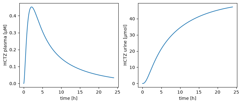
The result has every variable of the model at the time points the integrator chose: many where the curve changes fast, few where it is flat. _point counts them. res.q[...] gives a variable as a quantity, its values with their unit. [Cve_hctz] is the HCTZ concentration in the venous plasma, Aurine_hctz the amount excreted into the urine so far.

Quantities plot directly with matplotlib: the first quantity on an axis sets its unit, and label_axes writes the name and the unit of each axis. .to(...) converts a quantity into the unit you want to see:

fig, (ax1, ax2) = plt.subplots(1, 2, figsize=(9, 3.5))
ax1.plot(res.q["time"].to("hr"), res.q["[Cve_hctz]"].to("µM"))
label_axes(ax1, "time", "HCTZ plasma")
ax2.plot(res.q["time"].to("hr"), res.q["Aurine_hctz"].to("µmol"))
label_axes(ax2, "time", "HCTZ urine")

Output figure

Observables¶

Clinical studies report HCTZ in ng/ml and describe a curve by pharmacokinetic parameters, such as the peak concentration cmax. Observables compute both for every simulation. A Formula is an expression of model variables in the unit you ask for, and PK runs a non-compartmental analysis of a concentration:

from sbmlsim.simulation import PK, Formula

observables = [
    Formula("cp", "[Cve_hctz] * Mr_hctz", unit="ng/ml"),
    PK("pk", "cp", dose="PODOSE_hctz", route="oral"),
]
res = simulator.run(model, dose, observables)
units = {
    "pk.cmax": "ng/ml",
    "pk.tmax": "hr",
    "pk.auc_inf_obs": "ng*hr/ml",
    "pk.thalf": "hr",
}
for key, unit in units.items():
    print(f"{key:15} {res.q[key].to(unit):~.4g}")

Output

pk.cmax         134.6 ng / ml
pk.tmax         2.078 h
pk.auc_inf_obs  1253 h * ng / ml
pk.thalf        6.834 h

Mr_hctz is the molar mass of HCTZ, so cp is the mass concentration. The PK parameters come in the units of their timecourse and of the model, e.g. the peak time tmax in minutes, and .to(...) gives them in the units of a study.

Change the model¶

There are two kinds of changes. preinit_changes set values before the simulation starts, e.g. the body weight or the kidney function of a patient. A Change sets values at a time during the simulation, e.g. a dose. A Change with a list of times is a dosing regimen.

Here a patient with healthy kidneys and a patient with 30 % kidney function take 25 mg every day for a week:

def daily_dose(renal_function: float) -> Simulation:
    return Simulation(
        time_unit="hr",
        end=7 * 24,
        preinit_changes={"f_renal_function": renal_function},
        changes=[Change(range(0, 7 * 24, 24), {"PODOSE_hctz": Q(25, "mg")})],
    )


fig, ax = plt.subplots(figsize=(7, 3.5))
for renal_function in [1.0, 0.3]:
    res = simulator.run(model, daily_dose(renal_function), observables)
    label = f"renal function {renal_function}"
    ax.plot(res.q["time"].to("day"), res.q["cp"], label=label)
label_axes(ax, "time", "HCTZ plasma")
ax.legend(loc="upper left", bbox_to_anchor=(1, 1))

Output figure

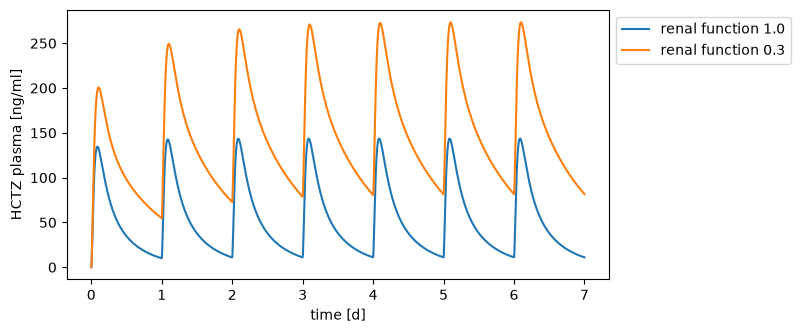
The kidneys remove HCTZ from the body. With 30 % kidney function the drug accumulates over the week.

Scan parameters¶

A Scan runs a simulation for every point of its Dimensions. A dimension maps parameters to arrays of values, and two dimensions give every combination of their values. The result is a labeled array with one axis per dimension:

from sbmlsim.simulation import Dimension, Scan

scan = Scan(
    dose,
    [
        Dimension(
            "dose",
            values={"PODOSE_hctz": Q([12.5, 25, 50, 100], "mg")},
            labels=["12.5 mg", "25 mg", "50 mg", "100 mg"],
        ),
        Dimension(
            "renal",
            values={"f_renal_function": [1.0, 0.5, 0.25]},
            labels=["normal", "mild", "severe"],
        ),
    ],
)
res = simulator.run(model, scan, observables)
print(res)
print(res["pk.cmax"].round(1).to_pandas())

Output

ScanResult(dose: 4, renal: 3, _point: 962; cp, pk.cmax, pk.tmax, pk.cmin, pk.tmin, pk.clast, pk.clast_pred, pk.tlast, ... (45 variables))
renal    normal   mild  severe
dose
12.5 mg    67.3   87.1   104.5
25 mg     134.6  174.1   208.9
50 mg     269.2  348.2   417.9
100 mg    538.4  696.5   835.8

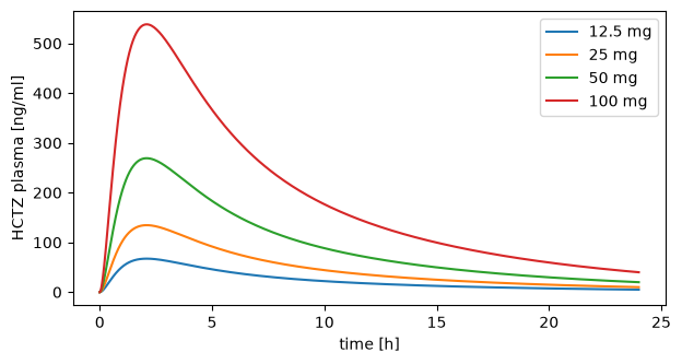
The values of the dose dimension replace the 25 mg of the Change. The peak concentration in ng/ml doubles with the dose, and it rises as the kidney function drops. Every simulation keeps its own time points, so time is a variable over _point and not one shared axis. sel selects points by their labels, here the curves of normal kidney function:

fig, ax = plt.subplots(figsize=(7, 3.5))
for label in res["dose"].values:
    point = res.sel(renal="normal", dose=label)
    ax.plot(point.q["time"].to("hr"), point.q["cp"], label=label)
label_axes(ax, "time", "HCTZ plasma")
ax.legend()

Output figure

A scan with many points runs in parallel on all cores. Parameter scans has the details.

Sensitivity analysis¶

Which parameters decide the exposure to the drug? A local sensitivity analysis changes each parameter by 1 % on its own and measures the relative change of the outputs. A value of 1 means the output changes in proportion to the parameter, -1 in inverse proportion. The design of the analysis is a dimension of a scan, so it runs like any other scan:

from sbmlsim import sensitivity
from sbmlsim.simulation import sampling

parameters = ["Ka_dis_hctz", "GU__F_hctz_abs", "KI__HCTZEX_k", "Kp_hctz", "BW"]
design = sampling.local(parameters, 0.01, model=model)
res = simulator.run(model, Scan(dose, [design]), observables)
local = sensitivity.local(res, observables=["pk.cmax", "pk.auc_inf_obs"])
print(local.index("normalized").to_pandas().round(2))

Output

observable      pk.cmax  pk.auc_inf_obs
parameter
Ka_dis_hctz        0.62            0.01
GU__F_hctz_abs     1.00            1.00
KI__HCTZEX_k      -0.42           -0.84
Kp_hctz           -0.45            0.00
BW                -1.10           -1.84

The fraction absorbed (GU__F_hctz_abs) scales the whole curve. The dissolution rate (Ka_dis_hctz) changes the peak but not the total exposure, the AUC. The excretion rate (KI__HCTZEX_k) lowers both. Body weight has the largest effect: in the model, organ volumes and blood flows grow with body weight, and so does the excretion by the kidneys, so a heavier patient has lower concentrations. Sensitivity analysis covers the global methods Sobol, FAST and Morris.

Fit the model to data¶

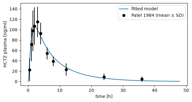
Patel et al. (1984) measured HCTZ in the plasma of 12 healthy volunteers after a 25 mg tablet. These are their means and standard deviations:

import pandas as pd

patel1984 = pd.DataFrame(
    {
        "time": [0.5, 1, 1.5, 2, 3, 4, 6, 8, 12, 24, 36],
        "cp": [22.8, 71.6, 97.9, 107, 115, 92.6, 54.2, 39.3, 23.3, 9.0, 4.6],
        "cp_sd": [21.9, 32.4, 39.1, 36.0, 29.0, 21.1, 11.6, 9.5, 11.9, 6.3, 5.2],
    }
)

A fit has to know which simulation belongs to which data. A SimulationExperiment describes a study: its models, datasets, simulations and tasks, where a task runs a simulation on a model. A FitMapping pairs a dataset with the simulated variable it measures:

from pathlib import Path
from typing import override

from sbmlsim.data import DataSet
from sbmlsim.experiment import SimulationExperiment
from sbmlsim.fit import FitData, FitMapping
from sbmlsim.task import Task


class Patel1984(SimulationExperiment):
    """A single oral dose of 25 mg HCTZ (Patel et al. 1984)."""

    @override
    def datasets(self) -> dict[str, DataSet]:
        units = {"time": "hr", "cp": "ng/ml", "cp_sd": "ng/ml"}
        return {"hctz25": DataSet.from_df(patel1984, udict=units)}

    @override
    def models(self) -> dict[str, Path]:
        return {"hctz": HCTZ_SBML}

    @override
    def simulations(self) -> dict[str, Simulation]:
        po25 = Simulation(
            time_unit="hr",
            end=48,
            changes=[Change(0, {"PODOSE_hctz": Q(25, "mg")})],
        )
        return {"po25": po25}

    @override
    def observables(self) -> dict[str, Formula]:
        return {"cp": Formula("cp", "[Cve_hctz] * Mr_hctz", unit="ng/ml")}

    @override
    def tasks(self) -> dict[str, Task]:
        return {"task_po25": Task(model="hctz", simulation="po25")}

    @override
    def fit_mappings(self) -> dict[str, FitMapping]:
        return {
            "fm_po25": FitMapping(
                self,
                reference=FitData(
                    self, dataset="hctz25", xid="time", yid="cp", yid_sd="cp_sd"
                ),
                observable=FitData(self, task="task_po25", xid="time", yid="cp"),
            )
        }

The fit estimates the dissolution rate and the excretion rate. A FitParameter names a model parameter with its bounds. run_optimization starts a local optimizer from random points within the bounds and collects the fits:

from sbmlsim.fit import FitMappingCollection, FitParameter
from sbmlsim.fit.optimization import OptimizationProblem
from sbmlsim.fit.runner import run_optimization

problem = OptimizationProblem(
    "hctz_fit",
    [FitMappingCollection(experiment=Patel1984)],
    [
        FitParameter(pid="Ka_dis_hctz", lower_bound=0.01, upper_bound=10, unit="1/hr"),
        FitParameter(pid="KI__HCTZEX_k", lower_bound=1e-5, upper_bound=1, unit="1/ml"),
    ],
)
fit = run_optimization(problem, size=5, seed=1, show_progress=False)
fitted = fit.parameter_set()
fitted_changes = {pid: Q(v, fitted.units[pid]) for pid, v in fitted.values.items()}
for pid, value in fitted_changes.items():
    print(f"{pid:13} {value:~.3g}")

Output

🚀 Optimization ────────────────────────────────────────────────────────────────

🎛 Parameters (2) ───────────────────────────────────────────────────────────────
parameter      start   lower   upper   unit
───────────────────────────────────────────
Ka_dis_hctz    -       0.01    10      1/hr
KI__HCTZEX_k   -       1e-05   1       1/ml
runs                5
workers             1 (serial)
converged           5/5 runs
best cost           425.867
optimizer time      0.2 s
Ka_dis_hctz   0.297 / h
KI__HCTZEX_k  0.00512 / ml

To compare the fitted model with the data, set the fitted values before the start of the simulation. The data become quantities as well, so they share the axes with the simulation:

fitted_dose = Simulation(
    time_unit="hr",
    end=48,
    preinit_changes=fitted_changes,
    changes=[Change(0, {"PODOSE_hctz": Q(25, "mg")})],
)
res = simulator.run(model, fitted_dose, observables)
time = Q(patel1984["time"].to_numpy(), "hr")
cp = Q(patel1984["cp"].to_numpy(), "ng/ml")
sd = Q(patel1984["cp_sd"].to_numpy(), "ng/ml")

fig, ax = plt.subplots(figsize=(7, 3.5))
ax.plot(res.q["time"].to("hr"), res.q["cp"], label="fitted model")
ax.vlines(time, cp - sd, cp + sd, color="black")
ax.plot(time, cp, "o", color="black", label="Patel 1984 (mean ± SD)")
label_axes(ax, "time", "HCTZ plasma")
ax.legend()

Output figure

A real fit combines many studies, with training and validation data, global optimizers and HTML reports. Parameter fitting explains these, and Identifiability shows how well the data determine each parameter.

Uncertainty analysis¶

The fitted values are estimates, and patients differ from each other. How sure is the prediction that weak kidneys raise the exposure? An Uncertain value is a value with a distribution. Here the body weight varies between patients (75 ± 12 kg), and both fitted parameters get an uncertainty of 30 %. An uncertain value goes where the value is used, e.g. into the simulation. Uncertain parameters go into an UncertaintyModel:

from sbmlsim.uncertainty import Uncertain, UncertaintyModel

weight = Uncertain(Q(75, "kg"), sd=Q(12, "kg"), kind="variability")


def patient(renal_function: float) -> Simulation:
    return Simulation(
        time_unit="hr",
        end=24,
        preinit_changes={"BW": weight, "f_renal_function": renal_function},
        changes=[Change(0, {"PODOSE_hctz": Q(25, "mg")})],
    )


uq = UncertaintyModel(
    parameters={pid: Uncertain(q, cv=0.3) for pid, q in fitted_changes.items()}
)

propagate draws the uncertain values, simulates every draw and summarizes the outputs. Both scenarios use the same draws, so they compare the same virtual patients. time= puts the concentrations of all draws on one grid of times, which the bands below need:

import numpy as np

from sbmlsim.uncertainty import propagate

uncertainty = propagate(
    model,
    {"healthy": patient(1.0), "impaired": patient(0.3)},
    uq,
    observables,
    outputs=["pk.cmax", "pk.auc_inf_obs"],
    n=1024,
    seed=1,
    time=Q(np.linspace(0, 24, 97), "hr"),
)
auc = uncertainty.summary(["pk.auc_inf_obs"])
print(auc[["scenario", "mean", "sd", "q0.05", "q0.95"]].round(0))
print(uncertainty.contributions("pk.auc_inf_obs", scenario="healthy").round(2))

Output

   scenario      mean       sd    q0.05     q0.95
0   healthy   66251.0  26028.0  33721.0  114597.0
1  impaired  193084.0  84094.0  90795.0  350917.0
       variable  index  correlated
0            BW   0.54       False
1  KI__HCTZEX_k   0.36       False
2   Ka_dis_hctz   0.00       False

contributions ranks the uncertain values by how much of the spread of the output each explains. The 5 % and 95 % quantiles of the concentration over all draws form a band:

from sbmlsim.sensitivity.uncertainty import plot_bands

fig, ax = plt.subplots(figsize=(7, 3.5))
for scenario, result in uncertainty.results.items():
    bands = result.summary(quantiles=[0.05, 0.5, 0.95])
    plot_bands(bands, "cp", ax=ax, label=scenario, time_unit="hr", name="HCTZ plasma")

Output figure

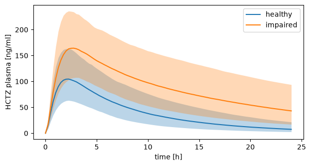
Last, test a statement about the prediction: in at least 90 % of the patients, does impaired kidney function raise the AUC by more than half?

from sbmlsim.uncertainty import Hypothesis

hypothesis = Hypothesis(
    "pk.auc_inf_obs", contrast=("impaired", "healthy"), greater=1.5, at_least=0.9
)
report = uncertainty.test([hypothesis])
print(report.table()[["hypothesis", "estimate", "low", "high", "decision"]])

Output

                                        hypothesis  estimate       low  high  decision
0  P(pk.auc_inf_obs:impaired/healthy > 1.5) >= 0.9       1.0  0.993154   1.0  accepted

The test takes the number of draws into account: with too few draws the decision is undecided. Uncertainty explains the statistics.

Next steps¶

Simulations: changes, events and outputs in detail.
Simulation experiments: studies as python classes, with figures and HTML reports.
Units: how sbmlsim reads and converts units.
PEtab: exchange a fit with other tools as a PEtab problem.