Gallery
Every figure of this page is written by one of the examples of the repository. An example is a module of the examples package and is run from the root of a checkout with python -m examples.<name>; it writes its figures into the working directory and never opens a window. The figures shown here are rendered by uv run python scripts/render_examples.py.
The snippet of a card is the core of its example. It runs from the root of a checkout, where the data of the example comes from its module (from examples.<name> import ...); the card links to the full source and to the page of the core functionality which explains the method.
-
Timecourses
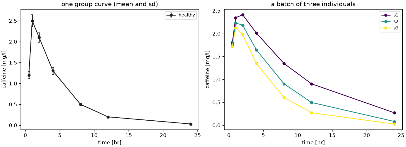
One curve with its dose, its units and the uncertainty of a group, and a batch of several curves over the sample dimensions.
-
NCA of one curve
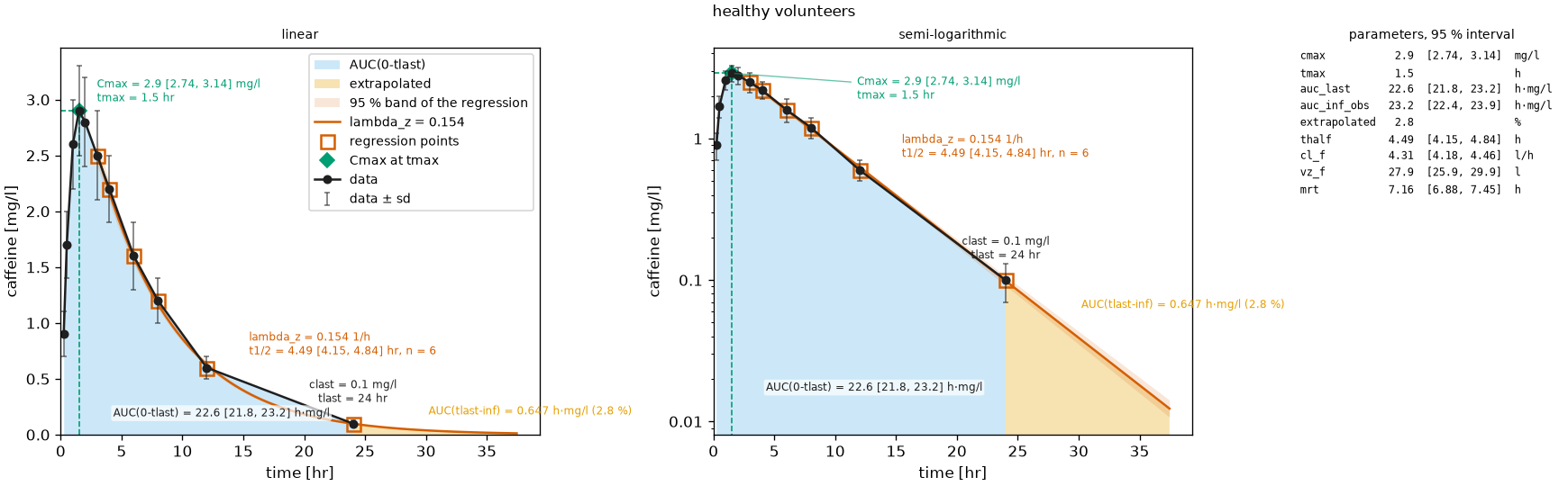
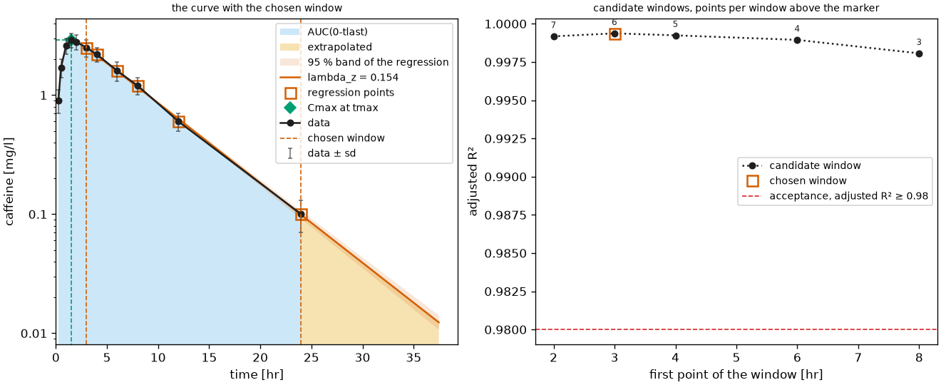
The non-compartmental analysis of a single timecourse with its diagnostic figure: the trapezoidal area, the extrapolated tail, the terminal regression with its confidence band and the parameters with their intervals; and the diagnostic of the terminal phase, every candidate window with its adjusted \(R^2\) and the chosen one marked.
from examples.nca_single import tc from pkpdutils import Acceptance, NCAOptions, TerminalPhase, nca_single from pkpdutils.plot import plot_nca, plot_terminal_windows result = nca_single(tc, options=NCAOptions(seed=1)) # a fixed bootstrap seed print(result.to_quantities()["auc_inf_obs"]) plot_nca(tc, result).savefig("nca_single.png", dpi=120) diagnostic = NCAOptions( terminal=TerminalPhase(keep_candidates=True), acceptance=Acceptance(r2_adj_min=0.98), ) windows = nca_single(tc, options=diagnostic) plot_terminal_windows(tc, windows, options=diagnostic).savefig( "nca_terminal_windows.png", dpi=120 ) -
NCA of a batch
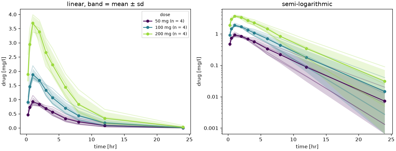
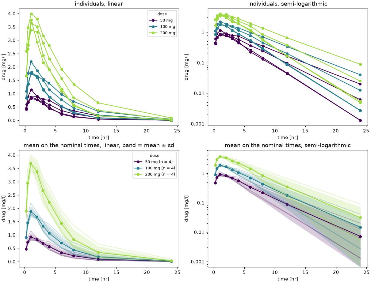
A
(dose, individual)batch analysed at once: the parameters of every curve as a data frame, the mean curve per dose group, a diagnostic panel per sample and the four panels a study report shows, the individuals on their actual sampling times and the means on the nominal ones.from examples.nca_batch import batch, study from pkpdutils import nca from pkpdutils.plot import plot_mean_timecourse, plot_nca_grid, plot_study_curves result = nca(batch) print(result.to_dataframe()[["dose", "individual", "auc_inf_obs", "cmax"]]) plot_mean_timecourse(batch, by="dose").savefig("nca_batch_curves.png", dpi=120) plot_nca_grid(batch, result, ncols=4).savefig("nca_batch.png", dpi=100) plot_study_curves(study, by="dose").savefig("nca_batch_study.png", dpi=110) -
Group uncertainty
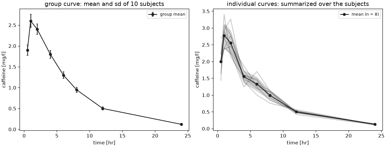
The uncertainty of a published mean curve propagated to the parameters with the bootstrap or the delta method, and individual results summarized over the subjects.
-
Multiple dosing and steady state
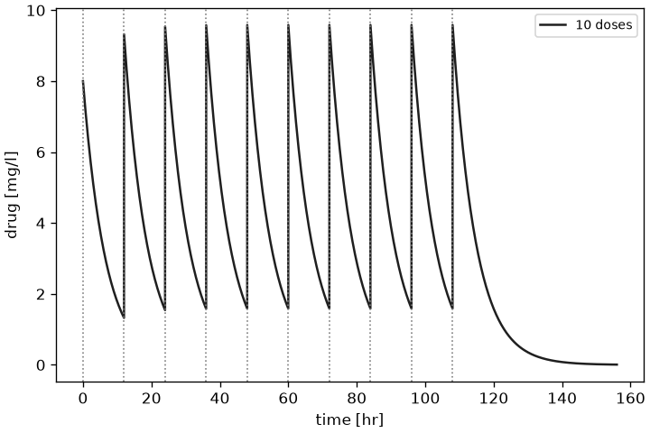
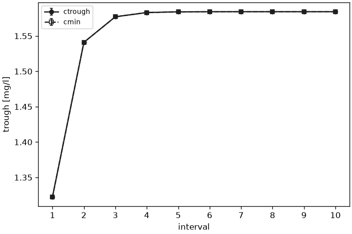
A single dose curve superposed into a regimen of ten doses, the parameters of every dosing interval and the steady state parameters of the last one, with the trough of every interval running into its plateau.
from examples.steady_state import single from pkpdutils import AUCMethod, Dose, Dosing, NCAOptions, Route, nca_single from pkpdutils.nca import superposition from pkpdutils.plot import plot_troughs dose = Dose(amount=100, unit="mg", route=Route.IV_BOLUS) protocol = Dosing.regimen(dose, interval=12, n_doses=10) options = NCAOptions(auc_method=AUCMethod.LOG) predicted = superposition(single, protocol, options=options) result = nca_single(predicted, options=options) print(result.to_quantities()["auc_tau"]) plot_troughs(result, x="interval").savefig("steady_state_troughs.png", dpi=120) -
Exchange formats
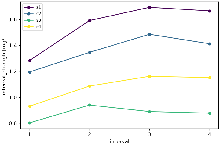
A twice daily batch written as event records and read back, analysed interval by interval;
from_adncareads a CDISC ADaM extract the same way.import pandas as pd from examples.formats import batch from pkpdutils import AUCMethod, NCAOptions, Route, Timecourses, nca from pkpdutils.plot import plot_intervals batch.to_events().to_csv("events.csv", index=False) read_back = Timecourses.from_events( pd.read_csv("events.csv"), time_unit="hr", unit="mg/l", dose_unit="mg", route=Route.ORAL, ) result = nca(read_back, options=NCAOptions(auc_method=AUCMethod.LOG)) plot_intervals(result, "interval_ctrough").savefig("formats.png", dpi=120) -
Exponential fitting
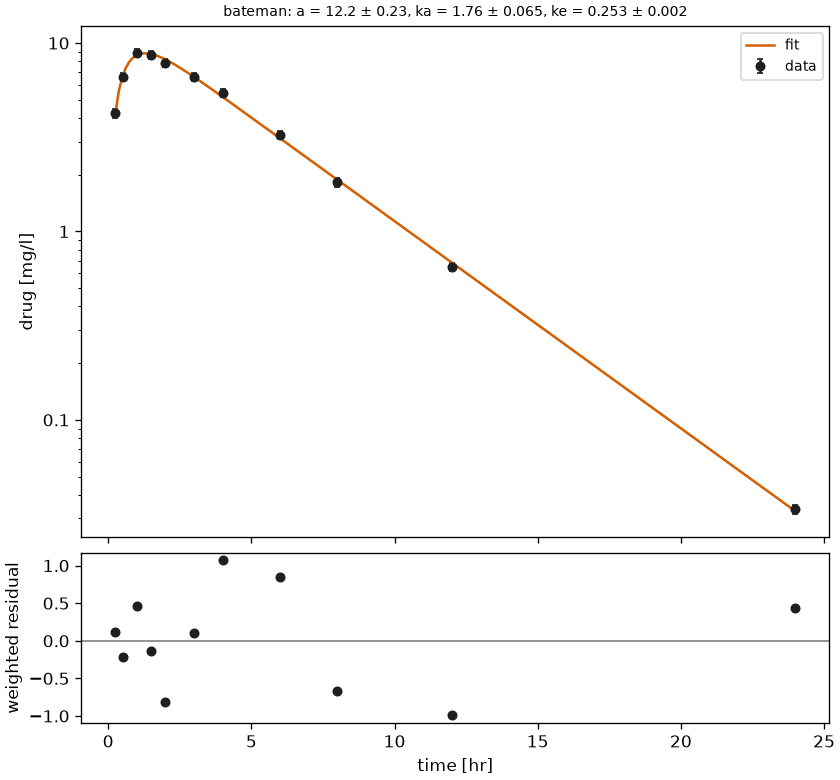
A Bateman model fitted to an oral curve with
1/sdweighting and a residual bootstrap, and the AICc comparison of the exponential models.from examples.fitting_exponential import tc from pkpdutils import Bateman, FitOptions, Weighting, fit_timecourse from pkpdutils.plot import plot_fit options = FitOptions(weighting=Weighting.INV_SD, n_starts=5, bootstrap=200, seed=1) result = fit_timecourse(Bateman(), tc, options=options) print(result.to_dataframe().T) plot_fit(result, log_y=True).savefig("fitting_exponential.png", dpi=120) -
Emax
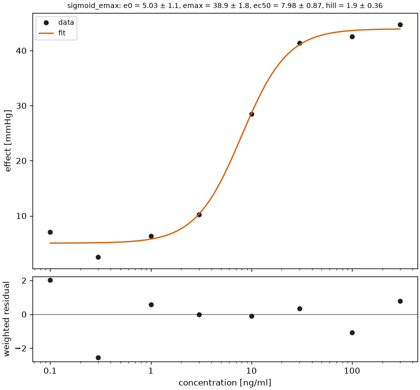
The concentration-effect relationship as a sigmoid Emax model, with
ec50,ec90and the comparison against the Emax and the linear model.from examples.emax import concentration, effect from pkpdutils import FitOptions, SigmoidEmax, fit from pkpdutils.plot import plot_fit result = fit( SigmoidEmax(), concentration, effect, x_unit="ng/ml", y_unit="mmHg", x_name="concentration", y_name="effect", options=FitOptions(n_starts=10, seed=0), ) print(result.to_quantities()["ec50"]) plot_fit(result, log_x=True).savefig("emax.png", dpi=120) -
Dose proportionality
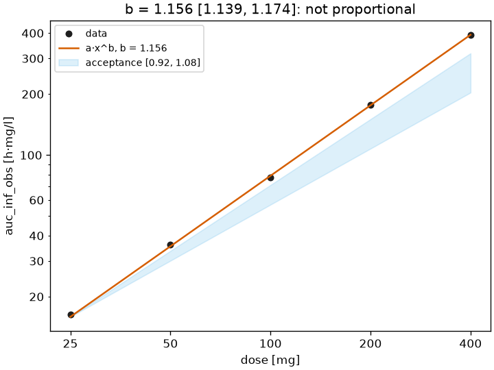
The power model \(AUC = a \cdot dose^b\) over a dose escalation and the confidence interval criterion of the dose proportionality.
from examples.dose_proportionality import batch, doses from pkpdutils import Power, fit_table, nca, proportionality_test from pkpdutils.plot import plot_dose_proportionality result = nca(batch) ds = result.ds.assign_coords(dose=("dose", doses, {"units": "mg"})) power = fit_table(Power(), ds, "dose", "auc_inf_obs", dim="dose") test = proportionality_test(power, dose_range=(25.0, 400.0)) print(test.slope, test.ci_low, test.ci_high, test.proportional) plot_dose_proportionality(power, test=test).savefig("dose_proportionality.png", dpi=120) -
Covariate and allometry
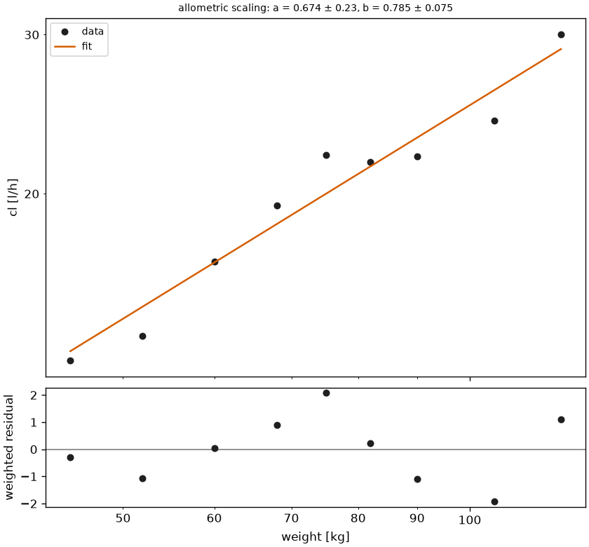
The clearance against the body weight as an allometric model, with a free exponent and with the exponent fixed at 0.75.
from examples.covariate import ds from pkpdutils import Allometric, fit_table from pkpdutils.plot import plot_fit free = fit_table(Allometric(), ds, "weight", "cl", dim="individual") print(free.to_dataframe().T.loc[["a", "b", "b_ci_low", "b_ci_high"]]) plot_fit(free, log_x=True, log_y=True).savefig("covariate.png", dpi=120) -
Bioequivalence
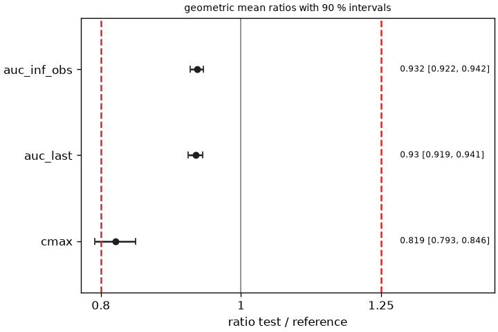
Average bioequivalence of a test against a reference formulation in a 2x2 crossover: the geometric mean ratios with their 90 % intervals against the 80-125 % limits.
from examples.bioequivalence import PERIOD_REF, PERIOD_TEST, batch, curves from pkpdutils import bioequivalence, nca from pkpdutils.plot import plot_ratio reference = nca(batch(curves(1.0, 1.5, PERIOD_REF), PERIOD_REF)) test = nca(batch(curves(0.93, 0.9, PERIOD_TEST), PERIOD_TEST)) result = bioequivalence(test, reference, parameters=["auc_inf_obs", "auc_last", "cmax"]) print(result.to_dataframe()[["parameter", "gmr", "ci_low", "ci_high"]]) plot_ratio(result).savefig("bioequivalence.png", dpi=120) -
Drug-drug interaction
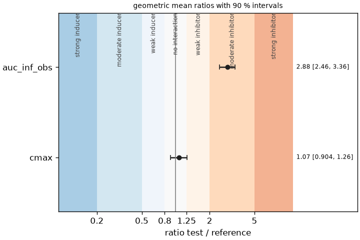
The exposure with and without a perpetrator as a geometric mean ratio, classified against the FDA and EMA thresholds of an interaction.
from examples.ddi import batch from pkpdutils import ddi_classification, nca, ratio from pkpdutils.plot import plot_ratio control = nca(batch(1.0, "control")) inhibited = nca(batch(0.35, "inhibitor")) auc = ratio( inhibited.sample("auc_inf_obs", "individual"), control.sample("auc_inf_obs", "individual"), ) print(ddi_classification(auc).to_dict()) plot_ratio({"auc_inf_obs": auc}, limits=None).savefig("ddi.png", dpi=120) -
Meta-analysis
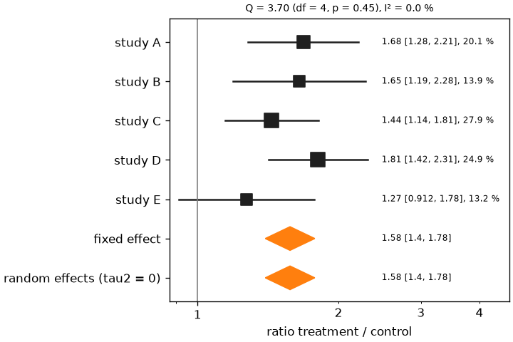
Published summary statistics of several studies pooled with the fixed effect and the random effects model, with the heterogeneity and a forest plot.
from examples.meta_analysis import STUDIES from pkpdutils import meta_analysis from pkpdutils.plot import plot_forest from pkpdutils.stats import EffectKind result = meta_analysis(STUDIES, EffectKind.LOG_RATIO) print(result.to_dataframe()) print(result.random.to_dict(), result.heterogeneity.i2) plot_forest(result).savefig("meta_analysis.png", dpi=120) -
Simulation scan
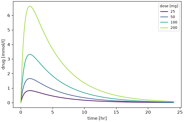
The result of a simulation scan read as a batch (
from_dataset,from_xresultfor an sbmlsimXResult) and analysed curve by curve.from examples.nca_from_sbmlsim import DOSES, simulated_dataset from pkpdutils import NCAOptions, Route, Timecourses, nca from pkpdutils.plot import plot_timecourse batch = Timecourses.from_dataset( simulated_dataset(), "[Cve]", unit="mmol/l", time_unit="hr", dose={"amount": DOSES, "unit": "mg"}, route=Route.ORAL, ) result = nca(batch, options=NCAOptions()) print(result.to_dataframe()[["dose", "auc_inf_obs", "cmax"]]) plot_timecourse(batch, by="dose").savefig("nca_from_sbmlsim.png", dpi=120) -
Urinary excretion
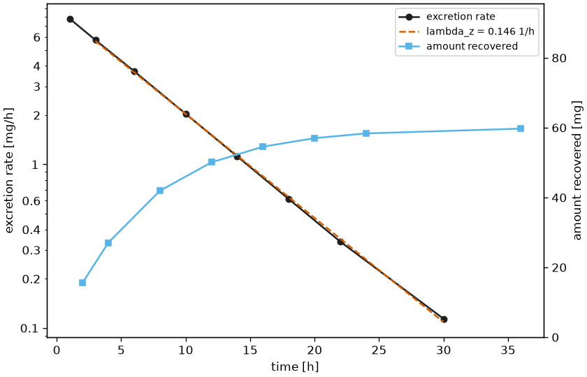
The excretion rate of every urine collection against the midpoint of its interval with the terminal regression, and the amount recovered rising to its plateau on a second axis.
-
Sparse sampling
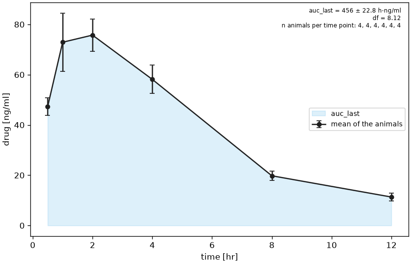
The mean curve of a destructive design with the standard error of every time point, the area the trapezoid rule integrates and the Bailer standard error of that area.
from examples.sparse import TIMES, serial_design
from pkpdutils import nca_sparse, sparse_mean
from pkpdutils.plot import plot_sparse

values = serial_design()
curve = sparse_mean(TIMES, values, time_unit="hr", unit="ng/ml")
result = nca_sparse(TIMES, values, time_unit="hr", unit="ng/ml")
plot_sparse(curve, result).savefig("sparse.png", dpi=120)
sparse.py · Sparse sampling - Study report
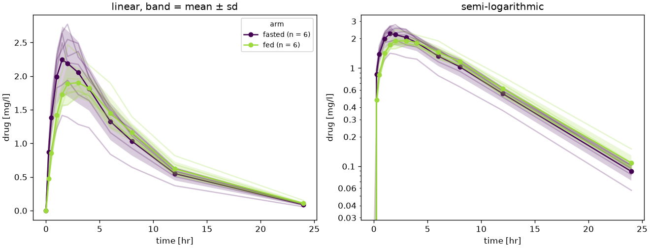
The tables and the figures of a study assembled into one self-contained HTML document: the methods sentence, the summary statistics of ICH M13A, the acceptability of the extrapolation, the parameters of every subject and the two figures.