Timecourses¶

A pharmacokinetic timecourse is the concentration of a substance in a tissue over time after a dose; a pharmacodynamic timecourse is an effect over time. pkpdutils represents one curve as a Timecourse and many curves as a Timecourses batch, which is the input of every analysis of the package. The first analysis is the non-compartmental analysis.

Concepts¶

Everything the package does starts at a Timecourse or a Timecourses batch, whichever way the data came in, and ends at a ParameterResult which the statistics and the figures read:

flowchart LR
  subgraph inputs["inputs"]
    ARR["arrays<br/>from_arrays"]
    DF["long table<br/>from_dataframe"]
    IO["event records / PKNCA / ADNCA<br/>pkpdutils.io"]
    SIM["simulation<br/>from_dataset, from_xresult"]
  end
  DOSE["Dose<br/>amount, unit, route, time, duration"]
  DOSING["Dosing<br/>amounts, times, durations<br/>single / from_doses / regimen"]
  TC["Timecourse<br/>time, value, sd, se, n<br/>units, metadata"]
  TCS["Timecourses<br/>xarray.Dataset, time + sample dims<br/>select, groupby, mean, dose_normalized"]
  NCA["nca / nca_single"]
  FIT["fit_timecourse / fit_timecourses / fit_table"]
  RES["ParameterResult<br/>NCAResult | FitResult<br/>summarize, summary_table"]
  PS["ParameterSample"]
  STATS["pkpdutils.stats<br/>compare, ratio, tost, ddi, meta"]
  PLOT["pkpdutils.plot"]

  DOSE --> DOSING --> TC
  ARR --> TCS
  DF --> TCS
  IO --> TCS
  SIM --> TCS
  TC -->|from_timecourses, to_batch| TCS
  TCS -->|sel / isel| TC
  TCS --> NCA --> RES
  TCS --> FIT --> RES
  RES -->|sample| PS --> STATS
  RES --> PLOT
  TCS --> PLOT

Single curve. A Timecourse holds the sampling times and the values with their units, an optional dose, and metadata (substance, label, tissue, the limit of quantification lloq of its assay). It is a frozen pydantic model: the arrays are converted to float64, sorted by time, and duplicate times or an unknown unit raise a ValueError when the object is created (a dimensionless value is spelled unit="dimensionless", the empty string is not a unit). Missing values are NaN in value; every analysis drops them. lloq travels into a batch as the coordinate lloq along its sample dimension, where the readers of Formats also write it, and the non-compartmental analysis reads it per sample when its options name no limit of their own.

Group data. Publications report the mean curve of a group with the standard deviation or the standard error and the number of subjects. A Timecourse carries these as sd, se and n; the missing one of sd and se is derived from the other with \(\mathrm{se} = \mathrm{sd}/\sqrt{n}\). The uncertainty analyses of the package propagate them to the parameters, see Uncertainty.

Doses and routes. A Dose has an amount with a dose unit (an amount or an amount per body weight, see Units), a Route, the time of the administration and, for an infusion, its duration. The route decides which parameters an analysis can report: after an intravenous bolus the clearance and the volume are absolute (cl, vz), after an extravascular dose they are relative to the unknown fraction absorbed (cl_f, vz_f), and an infusion shifts the mean residence time by half its duration. Route.ORAL stands for every extravascular route, and a route is also accepted as a string ("oral", "iv_bolus", ignoring the case). Either all or none of the curves of a batch carry a dose. A batch of curves which were given by one route carries it in attrs, and Timecourses.route returns it; curves of different routes travel in one batch as well, their routes becoming the coordinate route along the sample dimension, which Timecourses.routes reads back and the analysis follows per sample (Timecourses.route raises for such a batch). The substance works the same way: one substance in attrs and Timecourses.substance, several as the coordinate substance and Timecourses.substances, which is how a study of a parent and its metabolite is held in one batch, see Data formats.

Batches. Timecourses wraps an xarray dataset with a time dimension and any number of sample dimensions: the individuals of a study, the groups of a publication, the doses of a dose escalation, the dimensions of a simulation scan. Every analysis of the package is vectorized over the sample dimensions and returns a dataset over the same dimensions, so the parameters of a thousand curves are one call. Curves with different sampling times are stored per sample and padded with NaN, the times and values properties return the padded (samples..., time) arrays.

Repeated dosing. A timecourse is accompanied by its dosing protocol, not a single dose: the vector of the doses given and the times they were given, see Dosing protocols.

Dosing protocols¶

A Dosing is a frozen model of the doses given and the times they were given: amounts, times and durations (None unless the route is IV_INFUSION), one unit and one route for the whole protocol. The doses are sorted by time on construction and duplicate times raise. Dosing.single(dose) wraps a single Dose into a protocol of one, Dosing.from_doses(doses) builds one from a list of Dose objects sharing a unit and a route, and Dosing.regimen(dose, interval, n_doses) builds a regular protocol at dose.time + k * interval; DosingRegimen(dose=..., interval=..., n_doses=...).dosing() delegates to the same constructor and stays the convenient way to describe a regimen.

n_doses, doses (the protocol as a list of Dose), first and last (the first and the last Dose), intervals (np.diff(times)), tau (the common interval when every interval is equal within a relative tolerance, None for an irregular protocol or a single dose), is_regular, total_amount and shifted(offset) (a copy with every time shifted by -offset) read and transform a protocol.

Timecourse.dosing carries the protocol of one curve, None without dose information. The constructor also accepts a single dose: Dose keyword for backwards compatibility, converted into a protocol of one dose (giving both dose and dosing raises); Timecourse.dose is a read-only property returning the first dose of the protocol (or None), so tc.dose.amount, tc.dose.route and tc.dose.time keep working for a single dose curve. relative_to_dose(which="first" | "last") shifts the curve and its protocol so that the chosen dose is at time 0, which the non-compartmental analysis of a multiple dose curve uses to report the point parameters from the last dose on, see Non-compartmental analysis.

from pkpdutils import Dose, Dosing, DosingRegimen, Route, Timecourse

dose = Dose(amount=100, unit="mg", time=0, route=Route.ORAL)
protocol = Dosing.regimen(dose, interval=12, n_doses=4)  # 4 doses every 12 hr
same = DosingRegimen(dose=dose, interval=12, n_doses=4).dosing()
print(protocol.tau, protocol.total_amount)  # 12.0, 400.0

tc = Timecourse(
    time=[0.5, 1, 2, 11.5, 12.5, 13, 14, 23.5, 47.5],
    value=[0.9, 1.7, 2.6, 0.4, 1.0, 1.8, 2.5, 0.5, 0.2],
    time_unit="hr",
    unit="mg/l",
    dosing=protocol,
    substance="drug",
)
print(tc.dose.amount)  # the first dose, 100 mg
shifted = tc.relative_to_dose(which="last")
print(shifted.dosing.last.time)  # 0.0
print(shifted.dosing.first.time)  # -36.0

Data layout of a batch¶

Every variable carries attrs["units"]; the dataset carries substance, time_unit and unit in its attrs, tissue when the curves name one and route only when doses are present. Any further metadata (sex, body weight, study) is a coordinate on a sample dimension and travels with the results, so neither a coordinate nor a sample dimension may take the name of a variable of a result (cmax, n, flags) or of a dimension a result adds (interval and candidate of an NCA, point, parameter and parameter_ of a fit): the analysis raises a ValueError which names it. Several sample dimensions span their cartesian product: a combination without data is a sample of NaN values, which iteration and sel/isel return as a Timecourse with NaN values and without a dose. The dose dimension is called dose_index so that dose stays free as a sample dimension (the dose groups of a dose proportionality study, the dose axis of a simulation scan); a single dose batch has one dose column, and n_doses, first_dose_amount, last_dose_time and dosing_of read the protocol of a sample back.

API¶

A single curve:

from pkpdutils import Dose, Route, Timecourse

tc = Timecourse(
    time=[0.5, 1, 2, 4, 8, 12, 24],
    value=[1.2, 2.5, 2.1, 1.3, 0.5, 0.2, 0.03],
    sd=[0.3, 0.5, 0.4, 0.3, 0.1, 0.05, 0.01],
    n=12,
    time_unit="hr",
    unit="mg/l",
    dose=Dose(amount=100, unit="mg", route=Route.ORAL),
    substance="caffeine",
)
print(tc.se)  # derived from sd and n
print(tc.value_q)  # a pint quantity
print(tc.to_dataframe())

[0.08660254 0.14433757 0.11547005 0.08660254 0.02886751 0.01443376
 0.00288675]
[1.2 2.5 2.1 1.3 0.5 0.2 0.03] milligram / liter
   time  value    sd        se     n
0   0.5   1.20  0.30  0.086603  12.0
1   1.0   2.50  0.50  0.144338  12.0
2   2.0   2.10  0.40  0.115470  12.0
3   4.0   1.30  0.30  0.086603  12.0
4   8.0   0.50  0.10  0.028868  12.0
5  12.0   0.20  0.05  0.014434  12.0
6  24.0   0.03  0.01  0.002887  12.0

A batch from arrays, with the individuals as coordinate labels:

import numpy as np

from pkpdutils import Dose, Route, Timecourses

time = np.array([0.5, 1, 2, 4, 8, 12, 24])
values = np.random.default_rng(0).uniform(0, 3, size=(3, time.size))
tcs = Timecourses.from_arrays(
    time,
    values,
    time_unit="hr",
    unit="mg/l",
    dims=("individual",),
    coords={"individual": ["s1", "s2", "s3"]},
    dose=Dose(amount=100, unit="mg", route=Route.ORAL),
    substance="caffeine",
)
print(tcs.ds)
print(tcs.sel(individual="s2"))  # a Timecourse
for tc in tcs:  # iteration over the samples
    print(tc.label)

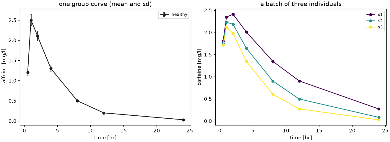
The curve with the uncertainty of its group and the batch of three individuals, as examples/timecourses.py builds them:

Doses and coordinates of a batch¶

dose= takes three forms. A single Dose or a single Dosing gives every sample of the batch the same protocol, as above. A mapping gives every sample its own doses, which is what a dose escalation, a crossover or a study with weight based dosing needs: amount (and time, duration) are arrays of the sample shape for one dose per sample, or of the shape (*sample_shape, n_dose) for one protocol per sample, padded with NaN; unit is the dose unit of the whole batch and the route is given by route=, since a mapping carries none.

import numpy as np
from pkpdutils import Route, Timecourses

time = np.array([0.5, 1, 2, 4, 8, 12, 24])
doses = np.array([50.0, 100.0, 200.0])
values = doses[:, None] / 40 * np.exp(-0.2 * time[None, :])
tcs = Timecourses.from_arrays(
    time,
    values,
    time_unit="hr",
    unit="mg/l",
    dims=("dose",),
    coords={"dose": doses},
    dose={"amount": doses, "unit": "mg"},  # one dose per sample
    route=Route.ORAL,
    substance="drug",
)
print(tcs.first_dose_amount, tcs.n_dose)

bid = np.tile(np.array([100.0, 100.0]), (3, 1))  # two doses per sample
tcs = Timecourses.from_arrays(
    time,
    values,
    time_unit="hr",
    unit="mg/l",
    dims=("dose",),
    coords={"dose": doses},
    dose={"amount": bid, "time": np.tile([0.0, 12.0], (3, 1)), "unit": "mg"},
    route=Route.ORAL,
)
print(tcs.n_doses)

[ 50. 100. 200.] 1
[2 2 2]

coords names the samples and carries everything else that is known about them: a non-dimension coordinate is given as (dimension, values) and travels through every analysis into the result, where summary_table(by=...), plot_timecourse(by=...) and the design detection of a bioequivalence study read it. The period and the sequence of a 2x2 crossover are exactly such coordinates, see Statistics:

coords = {
    "individual": ["s1", "s2", "s3"],
    "sex": ("individual", ["m", "f", "f"]),
    "weight": ("individual", [82.0, 61.0, 74.0]),
}

From a long table (one row per sample and time point) with a dose column, and from a list of Timecourse objects:

import pandas as pd
from pkpdutils import Route, Timecourse, Timecourses

df = pd.DataFrame(
    {
        "subject": ["a", "a", "a", "a", "b", "b", "b"],
        "time": [0.5, 1, 2, 4, 1, 4, 8],
        "value": [1.0, 2.0, 1.5, 0.8, 1.8, 1.0, 0.4],
        "dose": [50, 50, 50, 50, 100, 100, 100],
    }
)
tcs = Timecourses.from_dataframe(
    df,
    sample=["subject"],
    time_unit="hr",
    unit="mg/l",
    dose_amount="dose",
    dose_unit="mg",
    route=Route.ORAL,
)
print(tcs.sample_dims, tcs.sample_shape, tcs.first_dose_amount)

tc_a, tc_b = tcs.sel(subject="a"), tcs.sel(subject="b")
grouped = Timecourses.from_timecourses([tc_a, tc_b], dim="group")
one = tc_a.to_batch(dim="individual", label="s1")  # one curve as a batch of one
print(grouped.sample_shape, one.sample_shape)

('subject',) (2,) [ 50. 100.]
(2,) (1,)

The labels of the samples keep the dtype of what they came from: a subject column of integers gives an integer coordinate in from_dataframe, as the labels of from_timecourses do.

Timecourses.relative_to_dose(which="first" | "last") is the batch counterpart of Timecourse.relative_to_dose: every sample is shifted by the time of its own first (or last) dose, and its protocol with it. Equal shifts keep the layout of the batch; shifts which differ from sample to sample move the samples against each other, so the values are placed on the union of the shifted grids with NaN where a sample has no point at the time of another.

aligned = tcs.relative_to_dose()  # every first dose at time 0
last = tcs.relative_to_dose(which="last")  # `tcs`: the batch of the snippet above

Selecting, grouping and averaging a batch¶

A study arrives as one batch whose groups are coordinates on the individual dimension (the treatment, the dose group, the sex), so the four methods below cut the batch into the pieces an analysis or a figure needs. select keeps a batch (sel returns a single Timecourse and needs a label for every sample dimension), groupby walks the groups of a coordinate in the order of their first appearance, mean reduces a sample dimension to the group curve with its spread, and dose_normalized divides the values by the dose so that the curves of a dose escalation can be overlaid.

import numpy as np

from pkpdutils import Route, Timecourses

time = np.array([0.5, 1, 2, 4, 8, 12, 24])
rates = [0.20, 0.25, 0.18, 0.30]
values = np.stack([2.5 * np.exp(-k * time) for k in rates])
tcs = Timecourses.from_arrays(
    time,
    values,
    time_unit="hr",
    unit="mg/l",
    dims=("individual",),
    coords={
        "individual": ["s1", "s2", "s3", "s4"],
        "treatment": ("individual", ["test", "reference", "test", "reference"]),
        "weight": ("individual", [82.0, 61.0, 74.0, 95.0]),
    },
    dose={"amount": np.full(4, 100.0), "unit": "mg"},
    route=Route.ORAL,
    substance="drug",
)

arm = tcs.select(treatment="test")  # a label, a list of labels or a slice
heavy = tcs.select(weight=slice(80.0, 100.0))  # a coordinate along a sample dimension
print(arm.n_samples, heavy.n_samples)

for treatment, group in tcs.groupby("treatment"):
    print(treatment, group.n_samples)

group_curve = arm.mean("individual")
print(group_curve.values.round(3))
print(group_curve.ds["sd"].values.round(3), group_curve.ds["n"].values)

normalized = tcs.dose_normalized()  # values per dose amount
print(normalized.ds["value"].attrs["units"])

2 2
test 2
reference 2
[2.273 2.068 1.71  1.17  0.549 0.258 0.027]
[0.016 0.029 0.048 0.066 0.062 0.043 0.009] 2.0
1 / liter

mean(dim, spread="sd" | "se", min_n=1) averages the samples which have a finite value at a time point, carries their standard deviation and standard error and the count n of every time point, and sets a point covered by fewer than min_n samples to NaN. The count is the one of its own time point, so \(\mathrm{se} = \mathrm{sd}/\sqrt{n}\) holds everywhere, also on a ragged group whose late points carry fewer subjects than its early ones; n_subjects is the number of subjects of the group, the largest of the counts. The samples need a shared sampling grid; a ragged batch is placed on the union of its grids first, and relative_to_dose aligns samples which were dosed at different times. The group curve carries the dosing protocol of its samples when they share one and the protocol of the first sample with a warning when they do not; it is a Timecourses again, so nca propagates its spread to the parameters, see Uncertainty.

From a simulation: a dataset with a _time dimension and scan dimensions, with xres the XResult of a sbmlsim simulation and ds an xarray.Dataset shaped like one (examples/timecourses.py builds such a dataset in batch_from_simulation):

# not executed
tcs = Timecourses.from_xresult(
    xres, "[Cve_mid]", dose=Dose(amount=7.5, unit="mg", route=Route.IV_BOLUS)
)
tcs = Timecourses.from_dataset(ds, "[Cve]", unit="mmol/l", time_unit="min")

The complete example is examples/timecourses.py; the reference of the module is in API: timecourse.