Workflows
Five walk-throughs from the data of a study to the table and the figure a report prints. Every snippet runs on its own: copy it into a file, run it with python, and it writes the table to the console and the figure next to itself. The data is simulated in the first lines of every snippet so that nothing has to be downloaded; a real study replaces those lines with a read_csv and one of the readers. The same analyses on real fixtures are the runnable scripts of examples/, shown in the Gallery.
| workflow | question | output |
|---|---|---|
| A study from a table | what are the parameters of my study, per dose group? | the parameter table and the mean concentration-time figure |
| Bioequivalence | is the test formulation equivalent to the reference? | the ratio table with the 90 % intervals and the verdict |
| Drug-drug interaction | how strongly does the perpetrator change the exposure? | the ratio table with the interaction class |
| Multiple dosing and steady state | what does the curve look like at steady state? | the per-interval table, the steady state parameters and the trough figure |
| Dose proportionality | does the exposure grow in proportion to the dose? | the exponent with its interval and the acceptance wedge |
A study from a table
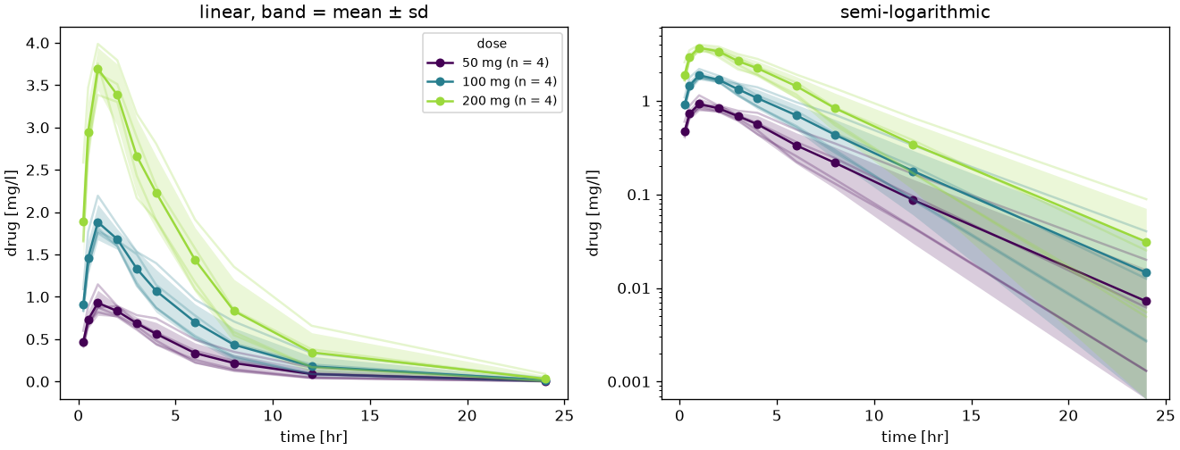
A parallel dose escalation: three dose groups of four subjects, one oral dose each, ten samples per subject. The study arrives as an event table (one row per dose and per sample, the layout of NONMEM and Monolix), from_events turns it into a batch of twelve curves with their dosing protocols, nca analyses all of them in one call, and summary_table writes the geometric mean and the geometric CV of every parameter per dose group.
import numpy as np
import pandas as pd

from pkpdutils import NCAOptions, Route, Timecourses, nca, summary_table
from pkpdutils.plot import plot_mean_timecourse

# the study as it arrives: one row per event (a dose or a sample), three dose
# groups of four subjects, the dose group as a column of its own
rng = np.random.default_rng(1)
time = np.array([0.25, 0.5, 1, 2, 3, 4, 6, 8, 12, 24])
ke = rng.uniform(0.15, 0.3, size=4)
ka = rng.uniform(1.0, 3.0, size=4)
records = []
for amount in (50.0, 100.0, 200.0):
    for j in range(4):
        curve = (
            amount
            / 40
            * ka[j]
            / (ka[j] - ke[j])
            * (np.exp(-ke[j] * time) - np.exp(-ka[j] * time))
            * rng.lognormal(0, 0.05, size=time.size)
        )
        group, subject = f"{amount:.0f}", f"{amount:.0f}-s{j + 1}"
        records.append(
            {
                "ID": subject,
                "TIME": 0.0,
                "DV": np.nan,
                "AMT": amount,
                "EVID": 1,
                "dose": group,
            }
        )
        records += [
            {"ID": subject, "TIME": t, "DV": c, "AMT": 0.0, "EVID": 0, "dose": group}
            for t, c in zip(time, curve, strict=True)
        ]
events = pd.DataFrame(records)
events.to_csv("study.csv", index=False)  # the table of the Quickstart
print(events.head())

# the table becomes a batch of twelve curves, each with its dosing protocol;
# a column which is constant within a subject becomes a coordinate
batch = Timecourses.from_events(
    events,
    time_unit="hr",
    unit="mg/l",
    dose_unit="mg",
    route=Route.ORAL,
    substance="drug",
    covariates=["dose"],
)

# every curve is analysed in one vectorized call
result = nca(batch, options=NCAOptions())

# the parameter table of the report: geometric mean and CV per dose group
print(
    summary_table(
        result,
        "individual",
        by="dose",
        parameters=["auc_inf_obs", "cmax", "thalf", "cl_f"],
        stats=("n", "geomean", "geocv"),
    ).to_string(index=False)
)

result.to_dataframe().to_csv("study_parameters.csv", index=False)
plot_mean_timecourse(batch, by="dose").savefig("study_curves.png", dpi=120)
The table this snippet builds is shipped with the documentation as study.csv, the file the Quickstart of the home page reads. Its first rows:
      ID  TIME        DV   AMT  EVID dose
0  50-s1  0.00       NaN  50.0     1   50
1  50-s1  0.25  0.412110   0.0     0   50
2  50-s1  0.50  0.661677   0.0     0   50
3  50-s1  1.00  0.872889   0.0     0   50
4  50-s1  2.00  0.890678   0.0     0   50
and the parameter table, one row per parameter and dose group:
| parameter | unit | dose | n | geomean | geocv |
|---|---|---|---|---|---|
| auc_inf_obs | hour * milligram / liter | 50 | 4 | 5.13 | 27.8 % |
| cmax | milligram / liter | 50 | 4 | 0.925 | 14.9 % |
| thalf | hour | 50 | 4 | 2.86 | 23.5 % |
| cl_f | liter / hour | 50 | 4 | 9.74 | 27.8 % |
| auc_inf_obs | hour * milligram / liter | 100 | 4 | 10.3 | 26.9 % |
| cmax | milligram / liter | 100 | 4 | 1.87 | 10.6 % |
| thalf | hour | 100 | 4 | 2.87 | 24.2 % |
| cl_f | liter / hour | 100 | 4 | 9.73 | 26.9 % |
| auc_inf_obs | hour * milligram / liter | 200 | 4 | 20.7 | 25.9 % |
| cmax | milligram / liter | 200 | 4 | 3.69 | 6.82 % |
| thalf | hour | 200 | 4 | 2.89 | 25.9 % |
| cl_f | liter / hour | 200 | 4 | 9.68 | 25.9 % |
The exposure triples with the dose while the clearance and the half-life stay where they are, which is what a linear dose range looks like; tmax in the same table would leave the two geometric columns empty, since a time read from the sampling grid carries no geometric statistics. study_curves.png is the concentration-time figure of the report, the mean of every dose group with the band of its standard deviation and the individual curves faint behind it, linear and semi-logarithmic:
Continue with Non-compartmental analysis for the parameters and the options, Data formats for the readers and Plotting for the figures.
Bioequivalence
A 2x2 crossover of a test against a reference formulation: twelve subjects, two periods, the sequences RT and TR. The period and the sequence of every subject are coordinates of the batch, they travel through the analysis, and bioequivalence recognizes the design from them and runs the two one-sided tests on the 90 % interval of the geometric mean ratio.
import numpy as np

from pkpdutils import Route, Timecourses, bioequivalence, nca
from pkpdutils.plot import plot_ratio
from pkpdutils.stats import ratio_table

# twelve subjects: sequence RT takes the reference in period 1 and the test in
# period 2, sequence TR the other way round; the test formulation has a lower
# bioavailability (0.93) and a slower absorption
time = np.array([0.25, 0.5, 1, 1.5, 2, 3, 4, 6, 8, 12, 24])
subjects = [f"s{i:02d}" for i in range(12)]
sequence = np.array(["RT"] * 6 + ["TR"] * 6)
period_test = np.where(sequence == "RT", 2, 1)
rng = np.random.default_rng(12)
subject_scale = rng.lognormal(0, 0.25, 12)  # between-subject variability


def period_batch(bioavailability: float, ka: float, period: np.ndarray) -> Timecourses:
    ke = 0.15
    scale = subject_scale * np.where(period == 2, 1.05, 1.0)  # period 2 runs higher
    values = np.stack(
        [
            s
            * bioavailability
            * 100
            * ka
            / (ka - ke)
            * (np.exp(-ke * time) - np.exp(-ka * time))
            / 30
            * rng.lognormal(0, 0.06, time.size)
            for s in scale
        ]
    )
    # the period and the sequence of every subject travel to the result as
    # coordinates along the individual dimension and make the design a 2x2
    return Timecourses.from_arrays(
        time,
        values,
        time_unit="hr",
        unit="mg/l",
        dims=("individual",),
        coords={
            "individual": subjects,
            "period": ("individual", period),
            "sequence": ("individual", sequence),
        },
        dose={"amount": np.full(12, 100.0), "unit": "mg"},
        route=Route.ORAL,
        substance="drug",
    )


reference = nca(period_batch(1.0, 1.5, 3 - period_test))
test = nca(period_batch(0.93, 0.9, period_test))

be = bioequivalence(test, reference, parameters=["auc_inf_obs", "auc_last", "cmax"])
print(ratio_table(be).to_string(index=False))
print("design:", be["cmax"].design, "| bioequivalent:", be.bioequivalent)

plot_ratio(be).savefig("bioequivalence.png", dpi=120)
| parameter | unit | n_test | n_reference | gmr | ci_low | ci_high | ci_level | cv_intra | limits | bioequivalent |
|---|---|---|---|---|---|---|---|---|---|---|
| auc_inf_obs | hour * milligram / liter | 12 | 12 | 93.0 % | 92.0 % | 94.0 % | 90 % | 1.47 % | 80.0 - 125.0 % | True |
| auc_last | hour * milligram / liter | 12 | 12 | 92.8 % | 91.7 % | 93.9 % | 90 % | 1.64 % | 80.0 - 125.0 % | True |
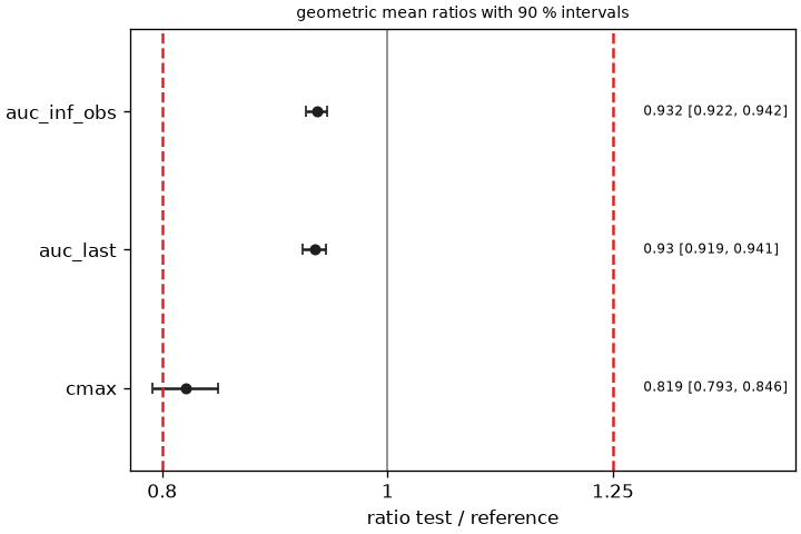
| cmax | milligram / liter | 12 | 12 | 81.9 % | 79.3 % | 84.6 % | 90 % | 4.39 % | 80.0 - 125.0 % | False |
design: crossover | bioequivalent: False: the exposure of the two formulations is equivalent, the peak is not, and a study is bioequivalent only when every parameter is. The figure puts the three ratios against the acceptance limits:
Continue with Bioequivalence for the designs, the two one-sided tests, the within-subject CV and the table of the report, and with Statistics for the samples and the intervals behind them.
Drug-drug interaction
The substrate is given alone and with the perpetrator; the exposure ratio of the two arms is classified against the thresholds of the FDA and the EMA guidelines. Here the two arms are parallel groups, so the ratio is a Welch interval on the log scale; a crossover would be paired by subject, which ratio does on its own when the labels match.
import numpy as np

from pkpdutils import Route, Timecourses, ddi_classification, nca, ratio
from pkpdutils.plot import plot_ratio
from pkpdutils.stats import DDIThresholds, ddi_table

# the substrate alone and with the perpetrator, two parallel groups of ten
# subjects; the inhibitor lowers the elimination of the substrate to 35 %
time = np.array([0.5, 1, 2, 4, 6, 8, 12, 24, 36, 48])
rng = np.random.default_rng(8)


def arm(clearance_factor: float, label: str) -> Timecourses:
    ke = 0.12 * clearance_factor
    values = np.stack(
        [
            rng.lognormal(np.log(8), 0.2)
            * np.exp(-ke * time)
            * rng.lognormal(0, 0.05, time.size)
            for _ in range(10)
        ]
    )
    return Timecourses.from_arrays(
        time,
        values,
        time_unit="hr",
        unit="mg/l",
        dims=("individual",),
        coords={"individual": [f"{label}{i}" for i in range(10)]},
        dose={"amount": np.full(10, 100.0), "unit": "mg"},
        route=Route.IV_BOLUS,
        substance="substrate",
    )


control = nca(arm(1.0, "control"))
inhibited = nca(arm(0.35, "inhibitor"))

# the exposure ratio with over without the perpetrator, and its class
auc_ratio = ratio(
    inhibited.sample("auc_inf_obs", "individual"),
    control.sample("auc_inf_obs", "individual"),
)
cmax_ratio = ratio(
    inhibited.sample("cmax", "individual"), control.sample("cmax", "individual")
)
ddi = ddi_classification(auc_ratio, cmax_ratio=cmax_ratio)
print(f"{ddi.strength} {ddi.kind}, uncertain: {ddi.uncertain}")

# the same over several parameters at once, one row each
print(
    ddi_table(inhibited, control, ["auc_inf_obs", "cmax"], dim="individual").to_string(
        index=False
    )
)

plot_ratio(
    {"auc_inf_obs": auc_ratio, "cmax": cmax_ratio},
    limits=None,
    thresholds=DDIThresholds.fda(),
).savefig("ddi.png", dpi=120)
moderate inhibitor, uncertain: False, and the table of both parameters:
| parameter | unit | n_test | n_reference | ratio | ci_low | ci_high | kind | strength | uncertain | source |
|---|---|---|---|---|---|---|---|---|---|---|
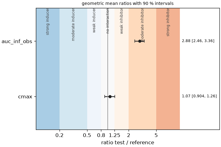
| auc_inf_obs | hour * milligram / liter | 10 | 10 | 2.88 | 2.46 | 3.36 | inhibitor | moderate | False | FDA 2020 |
| cmax | milligram / liter | 10 | 10 | 1.07 | 0.904 | 1.26 | none | none | True | FDA 2020 |
The exposure is raised almost threefold, a moderate inhibition; the peak of a bolus is not affected, and its interval spans the boundary at 1.25, which is what uncertain marks. The figure draws both ratios against the class boundaries:
Continue with Drug-drug interactions for the thresholds, the substrate sensitivity and the conservative reading of an interval, and with Statistics for the ratios behind them.
Multiple dosing and steady state
Four subjects on a twice daily regimen over two days, sampled in every dosing interval. The dosing protocol of the curves is what makes this a multiple dose analysis: nca splits every curve into its dosing intervals, reports the parameters of each of them, and describes the last complete interval with the steady state parameters.
import numpy as np

from pkpdutils import AUCMethod, Dose, Dosing, NCAOptions, Route, Timecourses, nca
from pkpdutils.nca import accumulation_ratio
from pkpdutils.plot import plot_intervals, plot_troughs

# four subjects on a twice daily oral regimen over two days, sampled in every
# dosing interval; the protocol is what makes this a multiple dose analysis
dose = Dose(amount=100, unit="mg", time=0, route=Route.ORAL)
protocol = Dosing.regimen(dose, interval=12, n_doses=4)
subjects = ["s1", "s2", "s3", "s4"]
offsets = np.array([0.5, 1, 2, 4, 8, 12])
time = np.concatenate([dose_time + offsets for dose_time in protocol.times])

rng = np.random.default_rng(3)
ke = rng.uniform(0.12, 0.18, size=4)
ka = rng.uniform(0.8, 1.2, size=4)
values = np.empty((4, time.size))
for j in range(4):
    elapsed = time[None, :] - protocol.times[:, None]
    single = (
        100.0
        / 20.0
        * ka[j]
        / (ka[j] - ke[j])
        * (np.exp(-ke[j] * elapsed) - np.exp(-ka[j] * elapsed))
    )
    values[j] = np.where(elapsed >= 0, single, 0.0).sum(axis=0) * rng.lognormal(
        0, 0.03, size=time.size
    )


def batch_of(times: np.ndarray, data: np.ndarray, dosing: Dose | Dosing) -> Timecourses:
    return Timecourses.from_arrays(
        times,
        data,
        time_unit="hr",
        unit="mg/l",
        dims=("individual",),
        coords={"individual": subjects},
        dose=dosing,
        route=Route.ORAL,
        substance="drug",
    )


options = NCAOptions(auc_method=AUCMethod.LOG)
result = nca(batch_of(time, values, protocol), options=options)

# one row per subject and dosing interval
print(
    result.intervals()[["individual", "interval", "interval_auc", "interval_ctrough"]]
    .head(8)
    .to_string(index=False)
)

# the steady state parameters describe the last complete interval
print(
    result.summary_table(
        "individual",
        parameters=["tau", "auc_tau", "cavg", "ctrough", "fluctuation"],
        stats=("n", "mean", "sd", "cv"),
    ).to_string(index=False)
)

# the accumulation, observed within the protocol and against the first interval
# analysed on its own as a single dose curve
first = time <= 12
single = nca(
    batch_of(time[first], values[:, first], dose),
    options=NCAOptions(auc_method=AUCMethod.LOG, tau=12),
)
print(result["accumulation_ratio_obs"].values.round(3))
ratios = accumulation_ratio(result, single)
print(ratios["accumulation_ratio"].values.round(3))
print(ratios["stationarity_ratio"].values.round(3))

plot_troughs(result, x="interval").savefig("troughs.png", dpi=120)
plot_intervals(result, "interval_ctrough").savefig("intervals.png", dpi=120)
The first two subjects of the per-interval table:
individual  interval  interval_auc  interval_ctrough
        s1         1     28.552763          1.283179
        s1         2     37.289613          1.591269
        s1         3     38.978011          1.693043
        s1         4     39.362381          1.665643
        s2         1     27.352591          1.194720
        s2         2     34.889015          1.345993
        s2         3     37.101878          1.485128
        s2         4     36.774156          1.412103
and the steady state parameters of the last interval over the four subjects:
| parameter | unit | n | mean | sd | cv |
|---|---|---|---|---|---|
| tau | hour | 4 | 12.0 | ||
| auc_tau | hour * milligram / liter | 4 | 34.3 | 4.62 | 13.5 % |
| cavg | milligram / liter | 4 | 2.86 | 0.385 | 13.5 % |
| ctrough | milligram / liter | 4 | 1.28 | 0.339 | 26.6 % |
| fluctuation | dimensionless | 4 | 1.15 | 0.197 | 17.2 % |
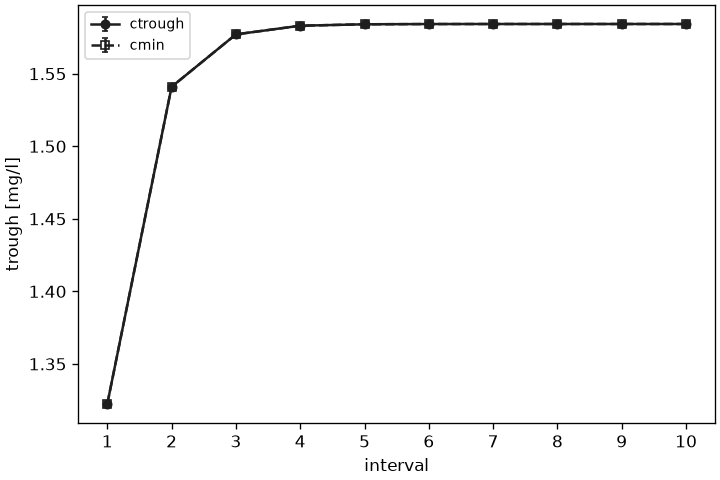
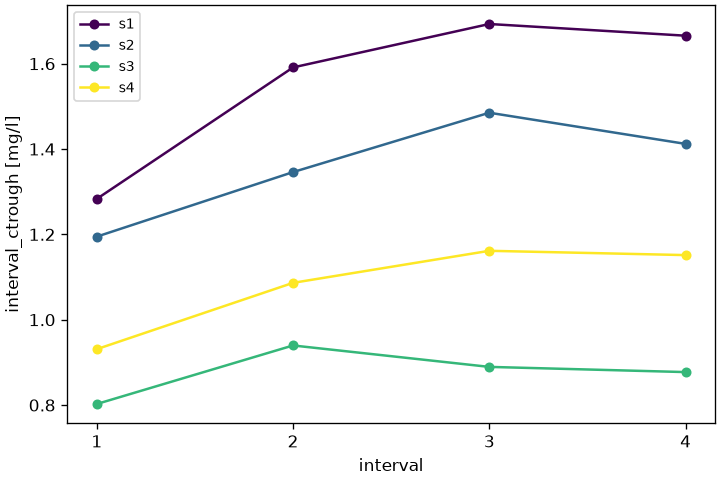
The area of the interval of the first subject grows from 28.6 to 39.4 over the four doses and levels off; over the four subjects the last interval carries [1.379 1.344 1.225 1.237] times the exposure of the first one, the observed accumulation accumulation_ratio_obs. accumulation_ratio(result, single) prints the same four numbers here as its accumulation_ratio, because the single dose analysis it compares against is the first interval of the same curves; with a separate single dose study it is the accumulation of that study against this one. Its second variable is the stationarity ratio \(\mathrm{AUC}_{0\text{-}\tau}^\mathrm{ss} / \mathrm{AUC}_{0\text{-}\infty}^\mathrm{single}\), [1. 1.003 1.017 1.001] here: the exposure over one interval at steady state is the total exposure of a single dose, which says that the clearance did not change over the study. troughs.png shows the mean trough of every dosing interval with its standard deviation over the subjects, 1.05, 1.24, 1.31 and 1.28 mg/l: the trough stops rising after the third interval, which is where steady state is reached. The same figure over a longer regimen, the ten doses of examples/steady_state.py, is the plateau itself:
plot_intervals of the same result draws one line per subject instead, the figure examples/formats.py writes for the same batch read back from its event records:
Continue with Non-compartmental analysis for the interval parameters, the reference dose rule and superposition.
Dose proportionality
A dose escalation over five doses: the exposure of every dose group goes into a power model \(\mathrm{AUC} = a D^b\), and the confidence interval criterion of Smith et al. decides whether the exponent is close enough to 1 over the dose range that was studied.
import numpy as np

from pkpdutils import Power, Route, Timecourses, fit_table, nca, proportionality_test
from pkpdutils.fit import proportionality_table
from pkpdutils.plot import plot_dose_proportionality

# a dose escalation whose exposure grows slightly faster than the dose
time = np.array([0.5, 1, 2, 4, 6, 8, 12, 24])
doses = np.array([25.0, 50.0, 100.0, 200.0, 400.0])
rng = np.random.default_rng(4)
values = np.stack(
    [
        d**1.15 / 10 * np.exp(-0.25 * time) * rng.lognormal(0, 0.04, time.size)
        for d in doses
    ]
)
batch = Timecourses.from_arrays(
    time,
    values,
    time_unit="hr",
    unit="mg/l",
    dims=("dose",),
    coords={"dose": doses},
    dose={"amount": doses, "unit": "mg"},
    route=Route.IV_BOLUS,
    substance="drug",
)

result = nca(batch)
# the dose coordinate of the result carries no unit, the fit needs one
ds = result.ds.assign_coords(dose=("dose", doses, {"units": "mg"}))
power = fit_table(Power(), ds, "dose", "auc_inf_obs", dim="dose")
test = proportionality_test(power, dose_range=(25.0, 400.0))
print(proportionality_table(test).to_string(index=False))

plot_dose_proportionality(power, test=test).savefig("dose_proportionality.png", dpi=120)
| slope | ci_low | ci_high | bound_low | bound_high | dose_low | dose_high | verdict |
|---|---|---|---|---|---|---|---|
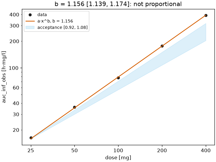
| 1.16 | 1.14 | 1.17 | 0.920 | 1.08 | 25.0 | 400 | not proportional |
The exponent is 1.16 with a narrow interval, the acceptance bounds of a sixteenfold dose range are 0.920 to 1.08, and the interval lies above them: the exposure grows faster than the dose. The figure draws the data, the fit and the acceptance wedge on log-log axes:
Continue with Curve fitting for the models, the weighting and the model comparison.