Statistics¶

Statistics on pharmacokinetic parameters: comparisons of two groups, geometric mean ratios, average bioequivalence, the classification of drug-drug interactions and the meta-analysis of published studies. Every function of pkpdutils.stats works on a ParameterSample, the values of one parameter over the individuals of a group or the summary statistics of the group, taken from an NCAResult or a FitResult with sample or typed in from a publication.

Concepts¶

Every analysis of this page starts at a ParameterSample, whether the numbers come from an analysis of the package or from a publication:

flowchart LR
  NR["NCAResult"] -->|"sample(name, dim, **indexers)"| PS
  FR["FitResult"] -->|"sample(name, dim, **indexers)"| PS
  PUB["published numbers<br/>ParameterSample(mean=, sd=, n=)<br/>or (geomean=, geocv=, n=)"] --> PS
  PS["ParameterSample<br/>values + labels + coords<br/>or summary moments"]
  PS --> SUM["summarize -> Summary"]
  PS --> CMP["compare -> TestResult<br/>t / Welch / rank / permutation"]
  PS --> RAT["ratio -> RatioResult (GMR, CI)<br/>ratio_table"]
  RAT --> DDI["ddi_classification -> DDIResult<br/>ddi_table"]
  PS --> TOST["tost / bioequivalence -> BEResult"]
  TOST --> DES{"Design detected"}
  DES --> X1["2x2 crossover<br/>(period + sequence coordinates)"]
  DES --> X2["paired (the same labels)"]
  DES --> X3["parallel"]
  PS --> ES["effect_size -> EffectSize"]
  ES --> META["meta_analysis<br/>fixed_effect, random_effects,<br/>heterogeneity"]
  CMP --> MC["multiple_comparison<br/>Holm / Bonferroni / BH"]

Log-normal parameters. Exposure, clearance, volume and half-life are positive and skewed: their logarithms are close to normal. The statistics therefore run on the log scale by default (Scale.LOG): differences of the logarithms are ratios of geometric means, intervals are symmetric on the log scale and asymmetric around the ratio, and the geometric mean and the geometric coefficient of variation \(\mathrm{CV}_g = \sqrt{e^{\sigma^2} - 1}\) describe a group. Scale.LINEAR compares arithmetic means, for parameters like \(t_\mathrm{max}\) or an effect which may be negative; summarize on Scale.LINEAR tolerates a non-positive value and reports geomean/geocv as NaN instead, while Scale.LOG raises on one.

Individual and summary data. With the individual values of a group every test of scipy is available; a publication often gives only the mean, the standard deviation and the number of subjects. A summary sample is analysed with the Welch t test from its moments; on the log scale the moments of the logarithm follow from the log-normal relations \(\sigma^2 = \ln(1 + \mathrm{sd}^2/\mathrm{mean}^2)\) and \(\mu = \ln\mathrm{mean} - \sigma^2/2\), or directly from the geometric mean and CV when they are reported.

Designs. In a parallel design two groups of different subjects are compared with the Welch interval. In a paired or crossover design every subject receives both treatments, and the within-subject differences remove the between-subject variability: the 2x2 crossover with its sequence, period and subject-within-sequence effects⁵ is the design of a bioequivalence study and is analysed on Bioequivalence.

Bioequivalence. Two formulations are bioequivalent when the 90 % confidence interval of the geometric mean ratio of \(\mathrm{AUC}\) and \(C_\mathrm{max}\) lies within 80-125 %¹, the two one-sided tests procedure of Schuirmann at \(\alpha = 0.05\)². The designs, the procedure, the within-subject CV and the table and figure of the report are on Bioequivalence.

Hodges-Lehmann. A rank test says whether two samples differ but reports no estimate of by how much. hodges_lehmann(a, b) adds it: the estimate is the median of the Walsh averages \((d_i + d_j)/2\) of the paired differences, or of the \(n_a n_b\) pairwise differences \(a_i - b_j\) of two independent samples, and the confidence interval is a pair of order statistics of the same quantities, taken at the quantile of the Wilcoxon signed rank or the Mann-Whitney null distribution⁸. The distribution is enumerated exactly up to fifty values per sample and approximated by its normal limit above, the p_value of the TestResult is the matching rank test of scipy, and the pairing is read from the labels unless paired= says otherwise. Because that distribution is discrete, an interval of order statistics rarely covers exactly what was asked for: TestResult.ci_level is the level it achieves, as R reports it (four pairs at a requested 0.90 reach 0.875). The analysis runs on the values as they are, not on their logarithms, because its use is \(t_\mathrm{max}\): a parameter read from a sampling grid, full of ties, not log-normal and not an acceptance parameter, which the EMA asks to be compared for its median and its variability when a rapid onset matters (see Bioequivalence).

Drug-drug interactions. A perpetrator is classified by how much it changes the \(\mathrm{AUC}\) of a sensitive substrate, a strong, moderate or weak inhibitor or inducer³⁴, read conservatively from the bound of the interval closer to 1. The thresholds, the sensitivity of a substrate and the table and figure of the report are on Drug-drug interactions.

Meta-analysis. Effects of several studies (Hedges' g, a mean difference or the log ratio of geometric means, the effect native to pharmacokinetics) are pooled with inverse variance weights¹². The fixed effect model assumes one true effect; the random effects model of DerSimonian and Laird adds the between-study variance \(\tau^2\) to every weight and widens the interval when the studies disagree⁷. \(Q\), \(I^2\) and \(H^2\) measure that disagreement⁹.

Math¶

Two-sample t tests. With the means \(\bar a\), \(\bar b\), the variances \(s_a^2\), \(s_b^2\) and the sizes \(n_a\), \(n_b\) (on the analysis scale), Welch's statistic is \(t = (\bar a - \bar b) / \sqrt{s_a^2/n_a + s_b^2/n_b}\) with the Welch-Satterthwaite degrees of freedom; Student's uses the pooled variance \(s_p^2 = ((n_a-1)s_a^2 + (n_b-1)s_b^2)/(n_a+n_b-2)\) with \(n_a + n_b - 2\); the paired test is the one-sample test of the differences. The interval of the effect is \(\hat\theta \pm t_{1-\alpha/2,\nu}\,\mathrm{se}\), exponentiated on the log scale. The standardized effect sizes are Cohen's \(d = (\bar a - \bar b)/s_p\) and Hedges' \(g = J d\) with \(J = 1 - 3/(4N - 9)\), \(N = n_a + n_b\)⁶. The rank tests (Mann-Whitney, Wilcoxon) and the permutation test report the same interval-free TestResult, with effect the difference or the ratio of the medians of the raw values for the rank tests: of the finite values of each sample for Mann-Whitney and of the remaining pairs for Wilcoxon. The estimate of the shift which belongs to the rank tests, with its distribution free interval, is hodges_lehmann.

Geometric mean ratio. Paired: \(d_i = \ln t_i - \ln r_i\), \(\ln\mathrm{GMR} = \bar d\), \(\mathrm{se} = s_d/\sqrt{n}\), \(n - 1\) degrees of freedom. Parallel: \(\ln\mathrm{GMR} = \bar{\ln t} - \bar{\ln r}\) with the Welch standard error. The interval of the ratio is \(\exp(\ln\mathrm{GMR} \pm t\,\mathrm{se})\). A paired ratio with no pair of finite values raises ValueError.

Pairing and degenerate samples. Paired analyses (compare(paired=True), ratio, tost) match the two samples with paired_values: by label when both samples carry labels, so the order of the individuals does not matter and an individual only one sample holds is dropped, and by position otherwise, which then needs equal sizes. A pair is dropped when either of its values is missing, which is logged at debug level; the analysis runs on the remaining pairs, so a missing parameter of one subject costs that subject and does not shift the pairing of the others. The statistic, the p value, the effect (the medians of the Wilcoxon test as well), its interval, Cohen's d, Hedges' g and n_a/n_b all come from those pairs. A sample of a single value and two samples without variance leave the statistic undefined: statistic, p_value, df and the interval come back as NaN instead of raising, while the effect itself (the difference or the ratio of the means) stays finite. A sample without a finite value at all (a parameter no subject of the group has) gives NaN throughout an unpaired compare or ratio and raises on a paired one, where no pair remains; tost reports NaN p values and no bioequivalence when the design leaves no standard error; effect_size gives a NaN effect and variance for such a group instead of raising, and the pooling drops that study with a warning naming it, keeps it with a NaN weight in MetaResult.to_dataframe and raises only when no study is left; a variance which is zero or negative is an error rather than a missing value, it carries an infinite weight and is named in a ValueError. ParameterSample rejects a negative sd or geocv, a non-positive geomean, an n which is not a whole number and a mix of the two kinds of data: summary fields next to values, which the statistics would never read, and labels or coords on summary data, which has no individuals.

Strings instead of enumeration members. Every option of pkpdutils.stats is taken either as its enumeration member or as the string of the member, so compare(a, b, scale="log", test="paired_t"), multiple_comparison(p, method="holm"), effect_size(control, treatment, "log_ratio") and tost(test, reference, design="parallel") run the analysis their members name. An unknown string raises a ValueError listing the members rather than falling back to a default.

The 2x2 crossover and the two one-sided tests. The period-difference analysis of a crossover, the within-subject CV and the equivalence of the two one-sided tests with the interval inclusion are on Bioequivalence; the thresholds and the conservative reading of an interval are on Drug-drug interactions.

Multiple comparisons. Bonferroni \(\tilde p_i = \min(1, m p_i)\); Holm sorts the p values and takes \(\tilde p_{(i)} = \max_{j \le i}\min(1, (m-j+1)p_{(j)})\)¹⁰; Benjamini-Hochberg takes \(\tilde p_{(i)} = \min_{j \ge i}\min(1, m p_{(j)}/j)\)¹¹.

Effect sizes of a study. Hedges' g as above with \(\mathrm{var}(d) = N/(n_C n_T) + d^2/(2N)\) and \(\mathrm{var}(g) = J^2\mathrm{var}(d)\); the mean difference \(\bar x_T - \bar x_C\) with \(s_T^2/n_T + s_C^2/n_C\); the log ratio \(\mu_T - \mu_C\) with \(\sigma_T^2/n_T + \sigma_C^2/n_C\).

Pooling. With \(w_i = 1/v_i\): \(\hat\theta_F = \sum w_i\theta_i/\sum w_i\), \(\mathrm{se} = 1/\sqrt{\sum w_i}\). Heterogeneity \(Q = \sum w_i(\theta_i - \hat\theta_F)^2\), \(C = \sum w_i - \sum w_i^2/\sum w_i\), \(\tau^2 = \max(0, (Q - (k-1))/C)\), \(I^2 = 100\max(0, (Q-(k-1))/Q)\) in percent, \(H^2 = Q/(k-1)\). Random effects: \(w_i^* = 1/(v_i + \tau^2)\) and the same pooling⁷⁹. The intervals of the effects and the pooled effects are normal, \(\hat\theta \pm z_{1-\alpha/2}\,\mathrm{se}\).

Results¶

The effect of compare is a - b on the linear scale and the ratio of the geometric means a / b on the log scale; ratio, tost and ddi_classification report test over reference and with over without the perpetrator. p_value of a BEParameter is the larger of the two one-sided p values, bioequivalent is p_value < (1 - ci_level) / 2, which is the interval within the limits.

Confidence levels and argument order. ci_level is 0.95 everywhere except ratio, tost, bioequivalence and ddi_table, which default to 0.90, the regulatory interval of the two one-sided tests: the 90 % interval of the ratio is the interval the bioequivalence decision reads². Every function takes ci_level as a keyword, so a comparison at another level is one argument away. The samples of a comparison are given test (or treatment) first: compare(a, b), ratio(test, reference), tost(test, reference), bioequivalence(test, reference); the meta-analysis reverses it, effect_size(control, treatment) and Study(label, control, treatment), the convention of its own literature⁶.

API¶

A sample comes from a result with sample(name, dim, **indexers), whose indexers name one label of every sample dimension besides dim, or from the numbers of a publication; summarize describes it, compare tests two of them against each other and ratio reports the geometric mean ratio with its 90 % interval:

import numpy as np

from pkpdutils import ParameterSample, Route, Timecourses, compare, nca, ratio
from pkpdutils.stats import Scale, summarize

# two parallel groups of eight subjects, smokers clear the drug 40 % faster
time = np.array([0.5, 1, 2, 4, 8, 12, 24])
rng = np.random.default_rng(5)


def group(ke: float, label: str) -> Timecourses:
    values = np.stack(
        [
            2.5
            * np.exp(-ke * rng.lognormal(0, 0.2) * time)
            * rng.lognormal(0, 0.05, time.size)
            for _ in range(8)
        ]
    )
    return Timecourses.from_arrays(
        time,
        values,
        time_unit="hr",
        unit="mg/l",
        dims=("individual",),
        coords={"individual": [f"{label}{i}" for i in range(8)]},
        dose={"amount": np.full(8, 100.0), "unit": "mg"},
        route=Route.IV_BOLUS,
        substance="drug",
    )


smokers = nca(group(0.28, "sm")).sample("cl", "individual")
non_smokers = nca(group(0.20, "ns")).sample("cl", "individual")

s = summarize(smokers)  # geometric mean with its interval, quantiles, CV
print(f"n={s.n} geomean={s.geomean:.4g} geocv={s.geocv:.3g}")
print(f"ci=[{s.ci_low:.4g}, {s.ci_high:.4g}] {s.unit}")
print(f"arithmetic mean {summarize(smokers, scale=Scale.LINEAR).mean:.4g}")

test = compare(smokers, non_smokers)  # Welch t on the log scale
print(test.test, round(test.p_value, 5), round(test.effect, 3), round(test.hedges_g, 2))
r = ratio(smokers, non_smokers)  # the same effect as a ratio with a 90 % interval
print(round(r.gmr, 3), round(r.ci_low, 3), round(r.ci_high, 3), r.paired)

published = ParameterSample(mean=45.2, sd=12.1, n=12, name="cl", unit="l/hr")
print(f"{compare(smokers, published).p_value:.3g}")  # Welch t from mean, sd, n

n=8 geomean=12.02 geocv=0.14
ci=[10.69, 13.5] liter / hour
arithmetic mean 12.12
welch_t 0.00115 1.403 1.96
1.403 1.214 1.621 False
5.08e-11

The effect of a comparison on the log scale is the ratio of the geometric means, so compare and ratio report the same 1.403 with different intervals: the 95 % interval of the test and the 90 % interval of the ratio.

The other tests, the pairing and the correction for multiple comparisons, with the samples of the snippet above and before/after two samples of the same subjects:

# not executed
from pkpdutils.stats import Alternative, TestMethod, multiple_comparison

compare(smokers, non_smokers, test=TestMethod.MANN_WHITNEY)
compare(before, after, paired=True, alternative=Alternative.LESS)
tests = [compare(smokers, non_smokers), compare(before, after, paired=True)]
multiple_comparison([t.p_value for t in tests])  # Holm

Ratios and bioequivalence, with test_result and reference_result two NCAResult objects of the same subjects:

# not executed
from pkpdutils import bioequivalence, ratio
from pkpdutils.stats import ratio_table

r = ratio(
    test_result.sample("auc_inf_obs", "individual"),
    reference_result.sample("auc_inf_obs", "individual"),
)  # paired by label when both carry the same subjects, 90 % interval
be = bioequivalence(test_result, reference_result, parameters=["auc_inf_obs", "cmax"])
be.bioequivalent, be["cmax"].gmr, be.to_dataframe()

ratio_table formats the ratios of a study the way a paper prints them: one row per parameter with the point estimate and its interval in percent of the reference (parameter, unit, n_test, n_reference, gmr, ci_low, ci_high, ci_level), the numbers rounded to digits significant digits as strings. It takes a mapping of RatioResult objects or the result of bioequivalence, which adds cv_intra, limits and bioequivalent.

# not executed
ratio_table(be)  # the table of a bioequivalence report
ratio_table({"auc_inf_obs": r}, percent=False, digits=4)  # plain ratios

The designs, the two one-sided tests, the within-subject CV and the table and figure of a study are on Bioequivalence, which runs the crossover above end to end.

Drug-drug interactions: ddi_classification classifies the exposure ratio of a substrate with and without a perpetrator, substrate_sensitivity grades the substrate against a strong inhibitor, and ddi_table does both over several parameters of two results. The thresholds, the conservative reading of an interval and the figure with the class bands are on Drug-drug interactions.

# not executed
from pkpdutils import ddi_classification
from pkpdutils.stats import DDIThresholds, ddi_table, substrate_sensitivity

# `inhibited` and `control`: the NCAResult of the two arms of the study
ddi = ddi_classification(
    ratio(
        inhibited.sample("auc_inf_obs", "individual"),
        control.sample("auc_inf_obs", "individual"),
    )
)
ddi.kind, ddi.strength, ddi.uncertain
ddi_classification(3.2, ci=(2.4, 4.3), thresholds=DDIThresholds.ema())
substrate_sensitivity(6.1)
ddi_table(inhibited, control, ["auc_inf_obs", "cmax"], dim="individual")

Meta-analysis:

import numpy as np

from pkpdutils import ParameterSample, meta_analysis
from pkpdutils.stats import EffectKind, Study, effects_from_arrays, random_effects

studies = [
    Study(
        "Smith 1990",
        control=ParameterSample(mean=1.2, sd=0.4, n=10),
        treatment=ParameterSample(mean=2.0, sd=0.6, n=10),
    ),
    Study(
        "Jones 1998",
        control=ParameterSample(mean=1.4, sd=0.5, n=24),
        treatment=ParameterSample(mean=2.1, sd=0.7, n=22),
    ),
    Study(
        "Meyer 2004",
        control=ParameterSample(mean=1.1, sd=0.3, n=16),
        treatment=ParameterSample(mean=2.4, sd=0.8, n=16),
    ),
]
meta = meta_analysis(studies, EffectKind.LOG_RATIO)
print(
    f"random effect {meta.random.estimate:.3f} "
    f"[{meta.random.ci_low:.3f}, {meta.random.ci_high:.3f}]"
)
print(
    f"fixed effect  {meta.fixed.estimate:.3f}, "
    f"tau2 {meta.heterogeneity.tau2:.4f}, I2 {meta.heterogeneity.i2:.1f} %"
)
print(meta.to_dataframe().round(4).to_string(index=False))

# effects computed elsewhere
pooled = random_effects(
    effects_from_arrays(
        np.array([0.51, 0.41, 0.78]),
        np.array([0.02, 0.01, 0.03]),
        labels=["Smith 1990", "Jones 1998", "Meyer 2004"],
        kind=EffectKind.LOG_RATIO,
    )
)
print(f"{pooled.estimate:.3f}, p = {pooled.p_value:.2e}")

random effect 0.566 [0.345, 0.788]
fixed effect  0.565, tau2 0.0255, I2 66.8 %
     label  estimate     se  ci_low  ci_high  n_control  n_treatment  weight_fixed  weight_random
Smith 1990    0.5204 0.1384  0.2492   0.7917         10           10        0.2134         0.2869
Jones 1998    0.4128 0.0990  0.2189   0.6067         24           22        0.4174         0.3629
Meyer 2004    0.7634 0.1052  0.5571   0.9696         16           16        0.3692         0.3502
0.530, p = 1.83e-07

The three studies agree on the direction and disagree on the size, which is what \(I^2 = 66.8\) % says: the random effects interval is wider than the fixed effect one would be, and the weights of the three studies are more even under it.

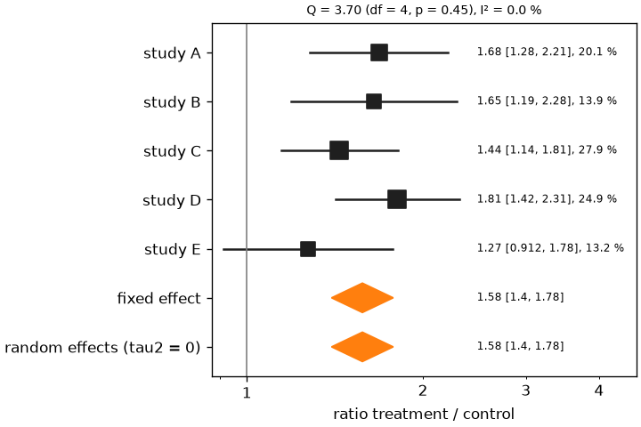
effects_from_arrays defaults to EffectKind.HEDGES_G like effect_size and meta_analysis, so the kind of an effect computed elsewhere is given explicitly. Every scalar result carries to_dict (Summary, TestResult, RatioResult, BEParameter, BEResult, EffectSize, PooledEffect, Heterogeneity, Study, MetaResult, DDIResult) and every collection a to_dataframe (BEResult, MetaResult).

Figures: plot_parameters, plot_ratio and plot_forest, see Plotting. Examples: examples/bioequivalence.py, examples/ddi.py and examples/meta_analysis.py. The reference of the modules is in API: stats, API: stats.bioequivalence, API: stats.ddi and API: stats.meta.

References¶