Non-compartmental analysis
Non-compartmental analysis (NCA) describes a concentration timecourse by parameters computed directly from the measured points, without a model of the body: the exposure as the area under the curve, the peak, the terminal half-life, and, with the dose, the clearance and the volume of distribution. pkpdutils.nca computes these parameters for one curve or for a whole batch of curves in one vectorized call; every parameter carries its unit and every sample carries flags for the conditions that limit its interpretation. The definitions follow Gabrielsson & Weiner 14 and the NCA of Phoenix WinNonlin 2, consistent with other open-source implementations such as NonCompart 5.
Concepts
Exposure. The area under the concentration–time curve, \(\mathrm{AUC}\), is proportional to the amount of drug that reached the systemic circulation 6. \(\mathrm{AUC}_{0\text{-}t_\mathrm{last}}\) is measured up to the last quantifiable concentration \(C_\mathrm{last}\); \(\mathrm{AUC}_{0\text{-}\infty}\) adds the tail after \(t_\mathrm{last}\), predicted from the terminal phase. The fraction of \(\mathrm{AUC}_{0\text{-}\infty}\) that is extrapolated tells how much of the exposure was not observed; above 20 % the estimate is considered unreliable (flag EXTRAPOLATION_HIGH).
Peak. \(C_\mathrm{max}\) and \(t_\mathrm{max}\) are read from the observed points. After an extravascular dose they reflect the balance of absorption and elimination, and the time of the last sample before the first measurable value is the lag of the absorption, \(t_\mathrm{lag}\); after an intravenous bolus the concentration at time zero, \(C_0\), is not observed and is back-extrapolated from the first two points.
The \(C_0\) of a bolus. The back extrapolation needs two samples which decline, so C0Method.LOG_BACK_EXTRAPOLATION (the default) falls back to the first observed value when the row has fewer than two points, when one of the two values is not positive, when the second value is not below the first or when the second time is not after the first, the fallback chain of Phoenix WinNonlin2. C0Method.FIRST_VALUE always takes the first value and C0Method.NONE estimates nothing: \(C_0\) is NaN, no point is inserted at the dose and the areas start at the first sample. Which rule a sample took is the variable c0_method (0 none, 1 back extrapolation, 2 first value) and how much of the exposure the estimate contributes is auc_back_extrap_fraction, the area of the segment from the dose to the first sample over \(\mathrm{AUC}_{0\text{-}\infty}\) (aumc_back_extrap_fraction for the moment); both are 0 when the first sample is taken at the dose. The inserted point never enters the terminal regression. A single dose infusion which carries no sample at the dose time starts at 0 there instead of at an estimate of \(C_0\): "for extravascular and infusion single dose a concentration of zero is inserted at the dose time"2, so the areas of such a curve carry the triangle from the dose to its first sample. The extravascular half of that rule is deliberately not applied to the areas of the analysis: an extravascular curve whose first sample is after the dose starts at that sample, which is what pkpdutils has always done and what the regression reference of pkdb_analysis 0.3.1 holds; only a partial area (partial_auc, NCAOptions.partial_aucs) inserts the zero for an extravascular dose, because an interval which begins at the dose has to begin somewhere. The asymmetry is written down in Validation. A steady state interval starts at the value the curve has at the dose (the interpolated trough of the interval before it, the back-extrapolated \(C_0\) after a bolus), not at 0.
Terminal phase. When absorption and distribution are over, the concentration declines mono-exponentially, \(C(t) = C_\mathrm{last}\, e^{-\lambda_z (t - t_\mathrm{last})}\). The terminal rate constant \(\lambda_z\) is the slope of \(\ln C\) against \(t\) over the terminal points; the half-life is \(t_{1/2} = \ln 2 / \lambda_z\). Which points belong to the terminal phase is a judgement: the default BEST_FIT rule takes the window with the largest adjusted \(R^2\) among all windows of at least three points that end at \(t_\mathrm{last}\) and start after \(t_\mathrm{max}\), preferring more points when the adjusted \(R^2\) is equal within a tolerance, as Phoenix does. LAST_N, ALL_AFTER_TMAX (the rule of pkdb_analysis 0.3.1) and MANUAL are the alternatives. After an intravenous infusion no sample taken at or before the end of the infusion is a candidate of any window: the concentration still rises while the drug is given, so the first point a window may start at is the first sample strictly after \(t_\mathrm{dose} + T\), which is the rule of Phoenix WinNonlin2 and the only place where the route changes the selection. TerminalPhase.exclude_cmax (default True) restricts every window to start after \(t_\mathrm{max}\); with exclude_cmax=False the window start is unrestricted and every window of at least min_points points ending at \(t_\mathrm{last}\) is a candidate, including windows that begin before or at the maximum, which is how a curve that only rises reports POSITIVE_SLOPE instead of TOO_FEW_POINTS. How far the window reaches is the quality criterion every regulatory review asks for: the span \(\mathrm{span} = (t_\mathrm{last} - t_\mathrm{first}) / t_{1/2}\) (lambda_z_span, from lambda_z_t_first and lambda_z_t_last) counts the half-lives the regression covers, and a span below 2 flags the row SPAN_LOW: the half-life of such a curve is extrapolated from less than one doubling of the elimination and carries little information.
Clearance and volume. With the dose \(D\), the clearance \(\mathrm{CL} = D / \mathrm{AUC}_{0\text{-}\infty}\) is the volume of plasma cleared of drug per time and the volume of distribution \(V_z = \mathrm{CL} / \lambda_z\) is the apparent volume the dose would occupy at the plasma concentration. After an extravascular dose the fraction absorbed \(F\) is unknown and both are reported relative to it as \(\mathrm{CL}/F\) (cl_f) and \(V_z/F\) (vz_f). The mean residence time \(\mathrm{MRT} = \mathrm{AUMC}_{0\text{-}\infty} / \mathrm{AUC}_{0\text{-}\infty}\) is the average time a molecule stays in the body (after an infusion of duration \(T\), minus \(T/2\)); the steady state volume \(V_\mathrm{ss} = \mathrm{CL} \cdot \mathrm{MRT}\) is reported for intravenous doses. A dose of 0, the encoding of a placebo arm, makes none of them a quantity: \(\mathrm{CL}\), \(V_z\), \(V_\mathrm{ss}\), auc_inf_dn and cmax_dn are NaN there, which the analysis reports in a debug log and not with a flag, since a zero dose is a property of the data and not a finding of the analysis.
Multiple dosing. A curve accompanied by a dosing protocol of more than one dose, or analysed with NCAOptions.tau, is split into its dosing intervals \([t_k, t_{k+1}]\) and the last interval \([t_K, t_K + \tau]\), whose length \(\tau\) comes from the protocol (the distance of the last two doses) or from tau when it is given 3. Every interval is described the same way as the classic steady state interval below: the value at its start and at its end are interpolated and inserted, so a sample outside the interval adds no area and does not enter its \(C_\mathrm{max}\) or \(C_\mathrm{min}\); after an intravenous bolus an interval that starts before the first sample of the curve starts at the back-extrapolated \(C_0\). An interval whose end is not covered by the data is incomplete: its parameters, and the steady state parameters when it is the last interval, are NaN and the row is flagged INCOMPLETE_INTERVAL. A last interval whose last measurable sample falls short of the end by at most NCAOptions.tau_tolerance of \(\tau\) (10 % by default) is not given up: its exposure is completed with the terminal regression and the share which was extrapolated is reported as auc_tau_extrap_fraction ("The last sample a little short of \(\tau\)" below). A sample recorded exactly at the end of a bolus interval may already be the post-dose value of the next dose; when it lies above the last sample inside the interval, which no decline can do, the trough is instead the log-linear regression of the last (up to three) samples of the interval and the row is flagged EXTRAPOLATED_TROUGH.
Steady state. The steady state parameters describe the last complete interval, under the assumption that repeated dosing has reached a state where every interval looks the same: with linear kinetics \(\mathrm{AUC}_{0\text{-}\tau}\) at steady state equals the single dose \(\mathrm{AUC}_{0\text{-}\infty}\). The interval is described by the average concentration \(C_\mathrm{avg} = \mathrm{AUC}_{0\text{-}\tau} / \tau\), the trough \(C_\mathrm{trough} = C(\tau)\), the fluctuation, the swing, the clearance at steady state \(\mathrm{CL}_\mathrm{ss}\), and the accumulation ratio, predicted from the terminal phase or observed as the ratio of the exposure of the last and the first interval of the protocol (accumulation_ratio_obs, NaN for a single dose protocol or when the first interval is incomplete); accumulation_ratio_cmax_obs, accumulation_ratio_cmin_obs and accumulation_ratio_ctrough_obs are the same ratio of the peak, the minimum and the trough. Regulators differ on whether the low point of an interval is its smallest observed value or the value at its end2, so the fluctuation and the swing come in both forms: fluctuation and swing read \(C_\mathrm{min,ss}\), fluctuation_tau and swing_tau read \(C_\mathrm{trough}\), and ptr is the peak-trough ratio \(C_\mathrm{max,ss} / C_\mathrm{trough}\).
The reference dose. With more than one dose the point parameters (\(C_\mathrm{max}\), \(t_\mathrm{max}\), \(C_\mathrm{last}\), \(\mathrm{AUC}_{0\text{-}t_\mathrm{last}}\), the extrapolated areas, the terminal phase, \(\mathrm{MRT}\)) are computed from the last dose on: the values before it are dropped and the times are relative to it, the same analysis a single dose curve given with its last dose only would get. With one dose the reference dose is that dose and the analysis covers the whole curve.
No single dose quantities. That slice is not a single dose curve: it carries the exposure of every earlier dose as well, so dividing the dose by its area would report a clearance that is too low and a volume that is too small. A multiple dose analysis therefore reports \(\mathrm{CL}\), \(\mathrm{CL}/F\), \(V_z\), \(V_z/F\), \(V_\mathrm{ss}\), auc_inf_dn and cmax_dn as NaN; the clearance of such an analysis is \(\mathrm{CL}_\mathrm{ss} = D_K / \mathrm{AUC}_{0\text{-}\tau}\) (cl_ss, cl_ss_f after an extravascular dose) over the dosing interval. \(\mathrm{AUC}_{0\text{-}\infty}\), \(\mathrm{AUMC}_{0\text{-}\infty}\) and \(\mathrm{MRT}\) are reported and describe the exposure and the decline after the last dose, extrapolated with its terminal phase, not the single dose exposure of the substance. A single dose curve analysed with tau is a multiple dose analysis as well, so the same holds for it. The decision is taken per sample and not per batch, so a batch mixing single dose and multiple dose subjects reports \(\mathrm{CL}\)/\(\mathrm{CL}/F\) for its single dose samples and \(\mathrm{CL}_\mathrm{ss}\)/\(\mathrm{CL}_\mathrm{ss}/F\) for its multiple dose ones; it carries the union of the two sets of variables and every sample is NaN in the variables of the other path.
Routes. IV_BOLUS reports \(C_0\), \(\mathrm{CL}\), \(V_z\), \(V_\mathrm{ss}\); IV_INFUSION corrects the \(\mathrm{MRT}\) by half the duration; ORAL (any extravascular route) reports \(\mathrm{CL}/F\), \(V_z/F\) and the half maximum during absorption (cmax_half, tmax_half). A batch usually has one route; a batch which mixes them (the intravenous reference and the oral test of an absolute bioavailability study, the coordinate route along a sample dimension) is analysed per route, so that every sample reports the parameters of the route it was given and NaN in the parameters of the other.
Missing values and the limit of quantification. NaN values are dropped; a value below the limit of quantification is handled by the rule its position asks for (BLQRules, "BLQ rules" below), by default dropped as BLQHandling.NAN does, and the sample is flagged BLQ_TRUNCATED where a value was dropped or imputed. The limit is NCAOptions.lloq, or, when the options name none, the limit of the sample itself: the lloq of a Timecourse and the coordinate lloq of a batch, which the readers of Formats fill from the data (ADNCA ALLOQ), so that a study with two assays or two analytes is analysed with a limit per subject.
The whole analysis of a batch, from the values to the result, with the multiple dosing path on the right:
flowchart TD
  IN["Timecourses<br/>(N, n_time)"] --> MD{"more than one dose<br/>or NCAOptions.tau?"}
  MD -->|no| BLQ
  MD -->|yes| REF["reference dose<br/>drop the points before the last dose,<br/>times relative to it"]
  REF --> BLQ["lloq (options or per sample)<br/>BLQRules per position<br/>drop / keep / impute, flag BLQ_TRUNCATED<br/>(point parameters only)"]
  BLQ --> PACK["pack_valid<br/>the valid points to the front of every row"]
  PACK --> AUC["segment_areas<br/>linear / linear-up-log-down / log<br/>auc_last, aumc_last"]
  PACK --> PEAK["cmax, tmax, clast, tlast<br/>c0 back-extrapolated for a bolus"]
  PACK --> TERM["window_statistics<br/>every candidate window at once"]
  TERM --> PICK["TerminalPhase rule<br/>BEST_FIT | LAST_N | ALL_AFTER_TMAX | MANUAL"]
  PICK --> LZ["lambda_z, thalf, r2_adj, lambda_z_span<br/>flags POSITIVE_SLOPE, TOO_FEW_POINTS, SPAN_LOW"]
  AUC --> EXTRAP["auc_inf_obs / auc_inf_pred<br/>auc_extrap_fraction, mrt"]
  LZ --> EXTRAP
  EXTRAP --> DOSEP["cl / cl_f, vz / vz_f, vss<br/>auc_inf_dn, cmax_dn<br/>(single dose analysis only)"]
  MD -->|yes| IV["compute_intervals<br/>interval_auc, interval_cmax,<br/>interval_ctrough per interval<br/>(the raw values, no BLQ rule)"]
  IV --> SS["compute_steady_state<br/>the last complete interval,<br/>completed within tau_tolerance<br/>auc_tau, cavg, fluctuation(_tau), ptr, cl_ss,<br/>accumulation_ratio(_obs, _cmax_obs, ...)"]
  DOSEP --> OUT["NCAResult<br/>xarray.Dataset + attrs['units'] + flags"]
  PEAK --> OUT
  SS --> OUT
LZ --> OUTMath
Trapezoid rules on a segment from \((t_1, C_1)\) to \((t_2, C_2)\) with \(\Delta t = t_2 - t_1\) and \(L = \ln(C_1 / C_2)\):
The logarithmic rule is exact for a mono-exponential segment. AUCMethod.LINEAR_LOG (the default, "linear up/log down") uses the linear rule on rising and the logarithmic rule on falling segments7, the rule compared against alternative numerical integration schemes for the same problem89; LINEAR uses the linear rule everywhere (the rule of pkdb_analysis 0.3.1); LOG the logarithmic rule wherever both values are positive.
Terminal regression of \(y = \ln C\) on \(t\) over \(n\) points:
Extrapolation and moments, with the observed \(C_\mathrm{last}\) (auc_inf_obs) or the value of the regression line at \(t_\mathrm{last}\), \(\hat C_\mathrm{last} = e^{b - \lambda_z t_\mathrm{last}}\) (auc_inf_pred):
The same with \(\hat C_\mathrm{last}\) in place of \(C_\mathrm{last}\) gives the predicted variants (aumc_inf_pred, mrt_pred, cl_pred, vz_pred, vss_pred, the extrapolated fractions with the suffix _pred), and \(\mathrm{MRT}_\mathrm{last} = \mathrm{AUMC}_{0\text{-}t_\mathrm{last}} / \mathrm{AUC}_{0\text{-}t_\mathrm{last}} - T_\mathrm{inf}/2\) (mrt_last) is the mean residence time over the observed curve.
The area starts at the dose. A curve whose first sample comes after it gets the value at the dose inserted: \(C_0\) after a bolus, 0 after an infusion and after an extravascular dose, both of which start from nothing (Phoenix WinNonlin, "for extravascular and infusion single dose a concentration of zero is inserted at the dose time"). The inserted point enters the areas and never the terminal regression.
\(C_0\) after a bolus by log-linear back-extrapolation of the first two points \((t_1, C_1)\), \((t_2, C_2)\): \(C_0 = \exp\!\left(\ln C_1 - t_1 \frac{\ln C_2 - \ln C_1}{t_2 - t_1}\right)\); the point \((0, C_0)\) enters the areas.
Steady state over the last complete interval \([t_K, t_K + \tau]\) (the values at its bounds are interpolated, or, after a bolus, back-extrapolated at the start and log-linearly regressed at the end when a post-dose sample lies at it):
The same three measures read against the trough at the end of the interval instead of the smallest observed value, with the peak-trough ratio:
Effective half-life, the half-life a drug would need to have the mean residence time it has, \(t_{1/2,\mathrm{eff}} = \ln 2 \cdot \mathrm{MRT}\) (PKNCA pk.calc.thalf.eff13); for a mono-exponential drug it is the terminal half-life, for a multi-exponential one it is the shorter half-life which governs the accumulation.
Accumulation ratio, predicted from the terminal phase or observed within one protocol as the ratio of the last and the first dosing interval, of the exposure and of the peak, the minimum and the trough:
accumulation_ratio (pkpdutils.nca.steady_state) compares two separate results the same way, the steady state and the single dose analysis of the same dosing interval, and adds the stationarity ratio against the total exposure of the single dose:
Bioavailability, the dose normalized exposure of a test treatment over that of a reference treatment, absolute (f_abs) against an intravenous reference and relative (f_rel) against any other:
Superposition predicts the multiple dose curve as the sum of the single dose curve shifted to every dose time, scaled by the dose ratio, interpolated inside the observed range and extrapolated with \(\lambda_z\) beyond \(t_\mathrm{last}\); it assumes linear kinetics.
Parameters
| name | symbol | definition | unit | needs |
|---|---|---|---|---|
cmax, tmax |
\(C_\mathrm{max}\), \(t_\mathrm{max}\) | maximum observed value and its time | value, time | |
cmin, tmin |
\(C_\mathrm{min}\), \(t_\mathrm{min}\) | minimum observed value and its time | value, time | |
clast, tlast |
\(C_\mathrm{last}\), \(t_\mathrm{last}\) | last measurable (positive) value and its time | value, time | |
clast_pred |
\(\hat C_\mathrm{last}\) | the terminal regression at \(t_\mathrm{last}\), \(e^{b - \lambda_z t_\mathrm{last}}\), which auc_inf_pred extrapolates with2 |
value | \(\lambda_z\) |
tlag |
\(t_\mathrm{lag}\) | time of the last sample after the dose before the first measurable value, 0 when the first sample at or after the dose is already measurable2; a sample below the limit of quantification is one only under a rule which keeps or imputes it (BLQRules.ich_m13a(), pkanalix(), pumas()), the default drops it. NaN when no value is measurable |
time | ORAL |
c0 |
\(C_0\) | back-extrapolated value at time 0 | value | IV_BOLUS |
c0_method |
rule which produced \(C_0\): 0 none, 1 back extrapolation, 2 first value | – | IV_BOLUS |
|
cmax_half, tmax_half |
value closest to \(C_\mathrm{max}/2\) before the maximum and its time | value, time | ORAL |
|
auc_last |
\(\mathrm{AUC}_{0\text{-}t_\mathrm{last}}\) | area to the last measurable value | value·time | |
auc_all |
\(\mathrm{AUC}_\mathrm{all}\) | area to the last observation, the trailing zeros and the values a BLQ rule imputed included; equal to auc_last when the last observation is positive2 |
value·time | |
auc_inf_obs, auc_inf_pred |
\(\mathrm{AUC}_{0\text{-}\infty}\) | area extrapolated with the observed or predicted \(C_\mathrm{last}\) | value·time | \(\lambda_z\) |
auc_extrap_fraction, auc_extrap_fraction_pred |
\((\mathrm{AUC}_{0\text{-}\infty} - \mathrm{AUC}_{0\text{-}t_\mathrm{last}}) / \mathrm{AUC}_{0\text{-}\infty}\), with the observed or the predicted \(\mathrm{AUC}_{0\text{-}\infty}\) | – | \(\lambda_z\) | |
auc_back_extrap_fraction, auc_back_extrap_fraction_pred, aumc_back_extrap_fraction |
share of \(\mathrm{AUC}_{0\text{-}\infty}\) (observed or predicted; of \(\mathrm{AUMC}_{0\text{-}\infty}\)) the segment from the dose to the first sample contributes, 0 with a sample at the dose | – | IV_BOLUS |
|
aumc_last, aumc_all, aumc_inf, aumc_inf_pred |
\(\mathrm{AUMC}\) | first moment of the curve, to the last measurable value, to the last observation2 and to infinity, extrapolated with the observed or the predicted \(C_\mathrm{last}\) | value·time² | \(\lambda_z\) for _inf |
aumc_extrap_fraction, aumc_extrap_fraction_pred |
\((\mathrm{AUMC}_{0\text{-}\infty} - \mathrm{AUMC}_{0\text{-}t_\mathrm{last}}) / \mathrm{AUMC}_{0\text{-}\infty}\), observed or predicted2 | – | \(\lambda_z\) | |
mrt, mrt_pred |
\(\mathrm{MRT}\) | mean residence time, from the observed or the predicted extrapolation | time | \(\lambda_z\) |
mrt_last |
\(\mathrm{MRT}_\mathrm{last}\) | mean residence time over the curve to \(t_\mathrm{last}\), \(\mathrm{AUMC}_{0\text{-}t_\mathrm{last}} / \mathrm{AUC}_{0\text{-}t_\mathrm{last}}\)2 | time | |
thalf_eff |
\(t_{1/2,\mathrm{eff}}\) | effective half-life, \(\ln 2 \cdot \mathrm{MRT}\)13 | time | \(\lambda_z\) |
lambda_z |
\(\lambda_z\) | terminal rate constant | 1/time | ≥ 3 terminal points |
thalf |
\(t_{1/2}\) | terminal half-life | time | \(\lambda_z\) |
lambda_z_n_points, lambda_z_t_first, lambda_z_t_last, lambda_z_r2, lambda_z_r2_adj, lambda_z_intercept, lambda_z_stderr |
diagnostics of the regression (lambda_z_t_first and lambda_z_t_last are the first and the last point of the window; lambda_z_stderr is the standard error of the slope) |
–, time, time, –, –, – (\(\ln C\)), 1/time | \(\lambda_z\) | |
lambda_z_span |
half-lives the terminal phase covers, \((t_\mathrm{last} - t_\mathrm{first}) / t_{1/2}\); below 2 the row is flagged SPAN_LOW |
– | \(\lambda_z\) | |
cl, cl_f, cl_pred, cl_f_pred |
\(\mathrm{CL}\), \(\mathrm{CL}/F\) | clearance (_f: extravascular; _pred: from auc_inf_pred) |
dose/(value·time) → l/h | dose, \(\lambda_z\), single dose analysis |
vz, vz_f, vz_pred, vz_f_pred |
\(V_z\), \(V_z/F\) | terminal volume of distribution | dose/value → l | dose, \(\lambda_z\), single dose analysis |
vss, vss_pred |
\(V_\mathrm{ss}\) | steady state volume of distribution | dose/value → l | intravenous dose, single dose analysis |
auc_inf_dn, auc_inf_pred_dn, cmax_dn |
dose normalized exposure and peak | value·time/dose, value/dose | dose, single dose analysis | |
x_dn |
any parameter per dose, from NCAResult.dose_normalized ("Dose normalization" below) |
unit of x/dose |
dose | |
auc_tau |
\(\mathrm{AUC}_{0\text{-}\tau}\) | area over the last complete dosing interval | value·time | protocol (≥ 2 doses) or tau |
cmin_ss, cmax_ss, ctrough, cavg |
\(C_\mathrm{min,ss}\), \(C_\mathrm{max,ss}\), \(C_\mathrm{trough}\), \(C_\mathrm{avg}\) | minimum, maximum, value at the end, average over the last interval | value | protocol (≥ 2 doses) or tau |
fluctuation, swing, accumulation_ratio |
see Math | – | protocol (≥ 2 doses) or tau |
|
fluctuation_tau, swing_tau, ptr |
the fluctuation, the swing and the peak-trough ratio read against \(C_\mathrm{trough}\) instead of \(C_\mathrm{min,ss}\)2 | – | protocol (≥ 2 doses) or tau |
|
auc_tau_extrap_fraction |
share of \(\mathrm{AUC}_{0\text{-}\tau}\) which was extrapolated to complete an interval whose last sample fell short of its end, 0 for an interval the data covers2 | – | protocol (≥ 2 doses) or tau |
|
accumulation_ratio_obs |
\(R_\mathrm{obs}\) | observed accumulation, last over first interval | – | protocol of ≥ 2 doses, first interval complete |
accumulation_ratio_cmax_obs, accumulation_ratio_cmin_obs, accumulation_ratio_ctrough_obs |
the same ratio of the peak, the minimum and the trough of the interval | – | protocol of ≥ 2 doses, first interval complete | |
cl_ss, cl_ss_f |
\(\mathrm{CL}_\mathrm{ss}\), \(\mathrm{CL}_\mathrm{ss}/F\) | \(D_K / \mathrm{AUC}_{0\text{-}\tau}\) (_f: extravascular) |
→ l/h | protocol (≥ 2 doses) or tau, dose |
n_doses, tau |
\(K\), \(\tau\) | number of doses of the protocol and the length of the last interval | –, time | protocol (≥ 2 doses) or tau |
flags |
NCAFlag bits, see below |
– |
Volumes are reported in liter (per kilogram for doses per body weight), clearances in liter per hour; every other unit is derived from the units of the input. Effect timecourses (Kind.EFFECT) report e0, emax_obs, temax, tlast, auec_last, auec_baseline, emax_baseline and time_above instead, see Pharmacodynamics; with a protocol they additionally report auec_tau, emin_ss, emax_ss, eavg, time_above_tau, accumulation_ratio_obs, n_doses and tau, the effect analogues of the row above.
Per-interval parameters
A protocol of more than one dose additionally reports the parameters of every single dosing interval, over the extra dimension interval (NCAOptions.intervals, default True); NCAResult.intervals() returns them as one row per sample and interval, with interval_start, interval_end and, with dose amounts, interval_dose as columns.
| name | symbol | definition | unit |
|---|---|---|---|
interval_auc |
\(\mathrm{AUC}_{0\text{-}\tau,k}\) | area over the interval | value·time |
interval_cmax, interval_tmax |
\(C_\mathrm{max,k}\), \(t_\mathrm{max,k}\) | maximum of the interval and its time relative to the interval start | value, time |
interval_cmin |
\(C_\mathrm{min,k}\) | minimum of the interval | value |
interval_ctrough |
\(C_\mathrm{trough,k}\) | value at the end of the interval | value |
interval_c_start |
\(C_\mathrm{start,k}\) | value at the start of the interval, interpolated or observed (after a bolus the post-dose value; the pre-dose value of interval \(k\) is interval_ctrough of interval \(k-1\)) |
value |
interval_cavg, interval_fluctuation, interval_swing |
average, fluctuation and swing of the interval | value, –, – | |
interval_n_points |
number of samples the interval uses (a boundary sample counts for both neighbours) | – |
For effect timecourses the same interval carries interval_auec, interval_emax, interval_temax, interval_emin, interval_eavg and interval_time_above instead. The interval variables are point variables (an extra dimension) and are excluded from to_dataframe.
Flags: POSITIVE_SLOPE (the terminal regression does not decline; \(\lambda_z\) and everything derived from it is NaN), TOO_FEW_POINTS (no window with the minimal number of points), EXTRAPOLATION_HIGH, NO_MAX (the maximum is the last point), NO_ABSORPTION (the maximum is the first point of an extravascular curve), BLQ_TRUNCATED, NO_DATA (fewer than two points), DELTA_WINDOW_CHANGE (the delta method skipped points at which the terminal window moved, see Uncertainty), INCOMPLETE_INTERVAL (the last dosing interval is not covered by the data; its parameters and the steady state parameters are NaN), EXTRAPOLATED_TROUGH (the trough of at least one dosing interval of a bolus was regressed because the sample at the dose time carries the post-dose value), SPAN_LOW (the terminal phase covers fewer than two half-lives, lambda_z_span < 2), NOT_ACCEPTED (a threshold of NCAOptions.acceptance is not met, see "Acceptance criteria and exclusions" below), PARTIAL_EXTRAPOLATED (a named partial area reaches beyond the last measurable value and was completed with the terminal regression, see "Partial areas").
API
One curve:
from pkpdutils import Dose, Route, Timecourse, nca_single

tc = Timecourse(
    time=[0.25, 0.5, 1, 2, 4, 6, 8, 12, 24],
    value=[0.9, 1.7, 2.6, 2.8, 2.2, 1.6, 1.2, 0.6, 0.1],
    time_unit="hr",
    unit="mg/l",
    dose=Dose(amount=100, unit="mg", route=Route.ORAL),
    substance="caffeine",
)
result = nca_single(tc)
q = result.to_quantities()
print(f"{q['auc_inf_obs']:~P}")  # hour * milligram / liter
print(f"{q['cl_f']:~P}", f"{q['thalf']:~P}")
print(result.flags())
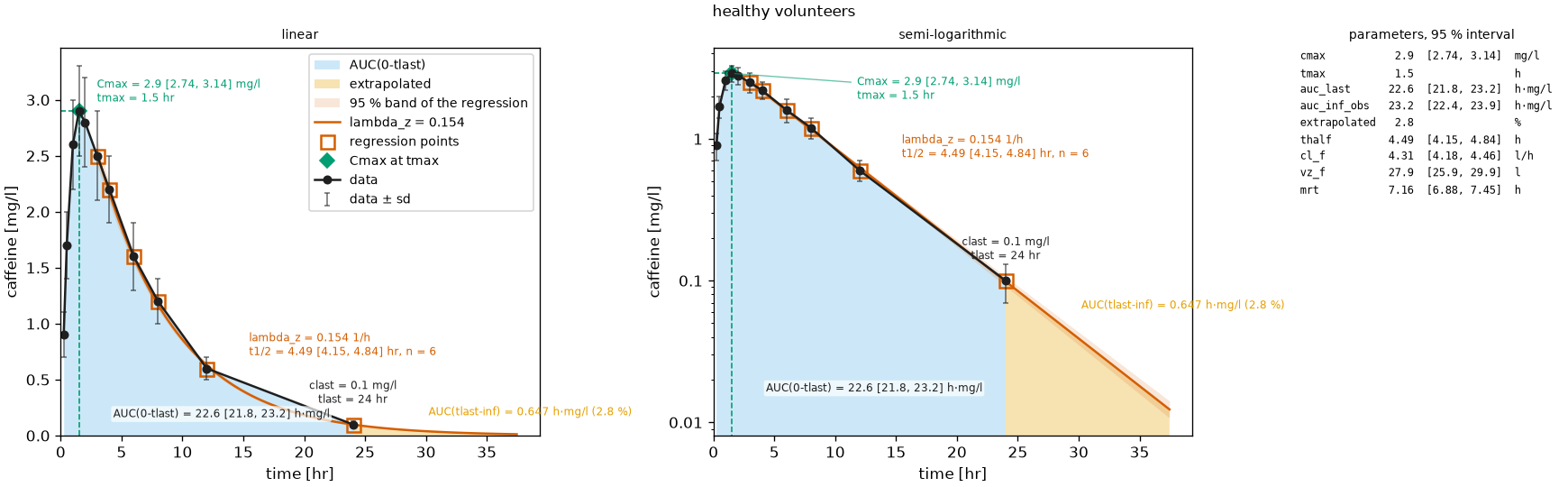
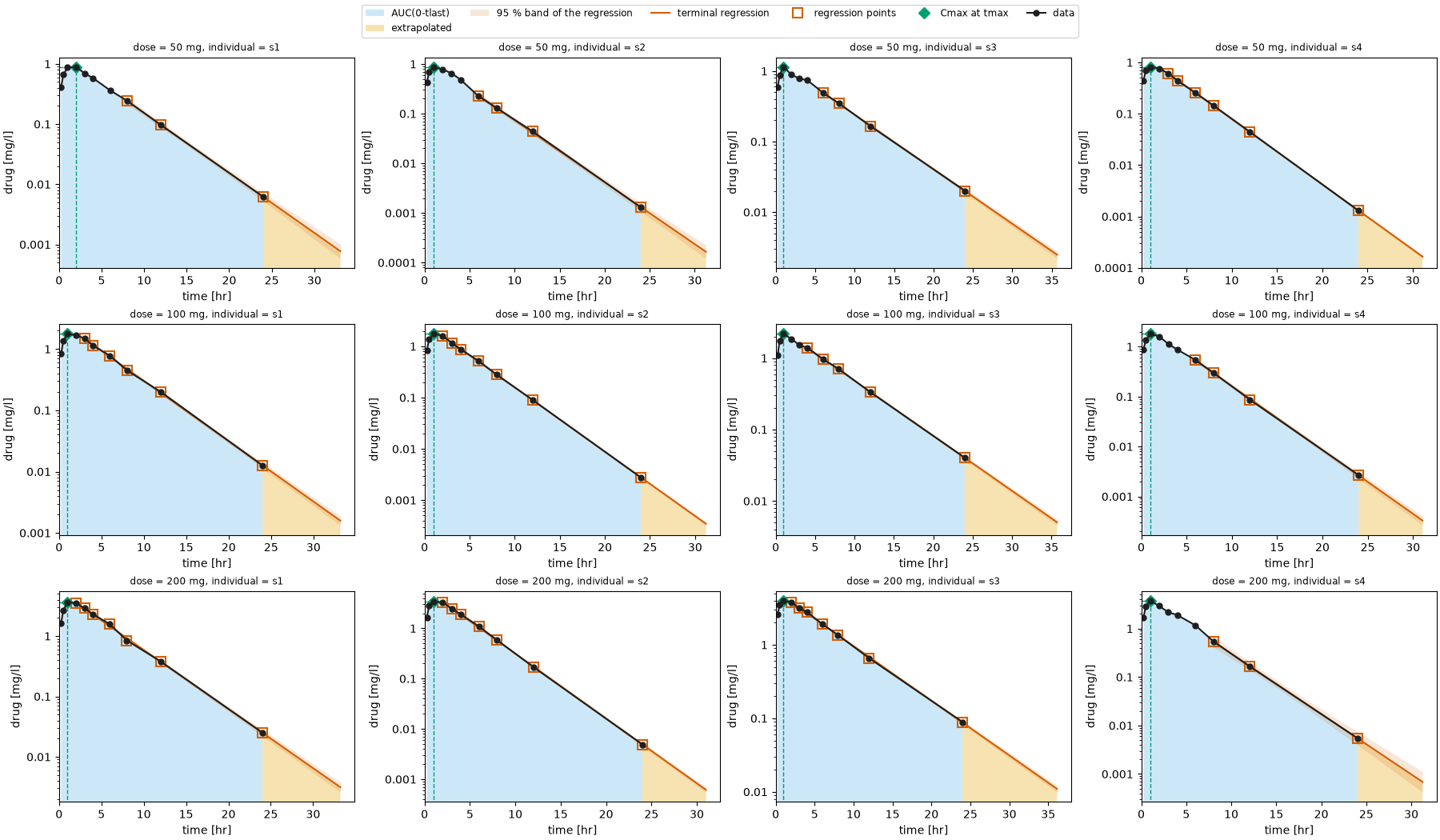
Options select the methods; the analysis of a batch returns the parameters over its sample dimensions. The batch below is the dose escalation of examples/nca_batch.py, four individuals at three dose levels:
import numpy as np

from pkpdutils import (
    AUCMethod,
    NCAOptions,
    Route,
    TerminalMethod,
    TerminalPhase,
    Timecourses,
    nca,
)

# a dose escalation: four individuals at three dose levels
rng = np.random.default_rng(1)
time = np.array([0.25, 0.5, 1, 2, 3, 4, 6, 8, 12, 24])
doses = np.array([50.0, 100.0, 200.0])
individuals = ["s1", "s2", "s3", "s4"]
ke = rng.uniform(0.15, 0.3, size=4)
ka = rng.uniform(1.0, 3.0, size=4)
values = np.stack(
    [
        np.stack(
            [
                d
                / 40
                * ka[j]
                / (ka[j] - ke[j])
                * (np.exp(-ke[j] * time) - np.exp(-ka[j] * time))
                * rng.lognormal(0, 0.05, size=time.size)
                for j in range(4)
            ]
        )
        for d in doses
    ]
)
batch = Timecourses.from_arrays(
    time,
    values,
    time_unit="hr",
    unit="mg/l",
    dims=("dose", "individual"),
    coords={"dose": doses, "individual": individuals},
    dose={"amount": np.broadcast_to(doses[:, None], (3, 4)), "unit": "mg"},
    route=Route.ORAL,
    substance="drug",
)

options = NCAOptions(
    auc_method=AUCMethod.LINEAR_LOG,
    terminal=TerminalPhase(method=TerminalMethod.BEST_FIT, min_points=3),
    lloq=0.001,
    extrapolation_warning=0.2,
)
result = nca(batch, options=options)
print(result["thalf"].dims, result["thalf"].attrs["units"])
print(
    result.to_dataframe()[
        ["dose", "individual", "auc_inf_obs", "cmax", "thalf", "cl_f", "flags"]
    ]
    .head(4)
    .to_string(index=False)
)
('dose', 'individual') hour
 dose individual  auc_inf_obs     cmax    thalf      cl_f flags
 50.0         s1     5.459071 0.890678 3.023747  9.159068
 50.0         s2     4.174637 0.874586 2.414383 11.977090
 50.0         s3     7.362814 1.146958 3.888391  6.790882
 50.0         s4     4.133924 0.818410 2.371655 12.095046
result.ds is the xarray.Dataset behind it, one variable per parameter over (dose, individual), and result.flag_table() is one boolean column per flag. plot_nca_grid(batch, result, ncols=4) draws the diagnostic panel of every sample of this batch:
BLQ rules
A value below the lower limit of quantification is not a measurement: the assay only says that it is below the limit. Which number the analysis puts in its place decides how much of the tail of the curve is counted as exposure, and the tools slice the profile on two incompatible axes to decide it. BLQRules expresses both, one rule per position, each BLQAction.DROP, KEEP, ZERO, LLOQ, HALF_LLOQ or a number to impute:
- by position:
first(before the first measurable value),middle(between two measurable values),last(after the last measurable value), as PKNCA13 and Pumas do; - by the maximum:
before_tmaxandafter_tmax, as PKanalix does.
A rule set uses one axis or the other, never both, and a position without a rule drops its values. The rules reach the point parameters of a curve, the ones computed from the reference dose on; the per-interval and the steady state parameters (interval_*, auc_tau, cavg, ctrough, cmin_ss) are computed from the values as they were measured, so no rule changes them. An imputed value enters the areas, so auc_all is where the imputation shows; a value which KEEP keeps is treated the same way. Neither is a quantified value, so neither becomes \(C_\mathrm{last}\) and neither enters the terminal regression unless terminal_regression=True asks for it, which is what ICH M13A11 requires: values below the limit are "treated as zero in PK parameter calculations" and "omitted from the calculation of kel and t½". The presets are BLQRules.ich_m13a(), BLQRules.pkanalix() and BLQRules.pumas(); the two classic values BLQHandling.NAN (the default, everything dropped) and BLQHandling.ZERO_BEFORE_TMAX stay and are the rule sets NCAOptions.blq_rules spells out.
import numpy as np

from pkpdutils import BLQRules, Dose, NCAOptions, Route, Timecourse, nca_single

# a curve whose last two samples are below the limit of quantification of 0.1
blq_curve = Timecourse(
    time=[0.0, 0.5, 1, 2, 4, 8, 12, 16],
    value=[0.02, 2.0, 4.0, 3.0, 1.5, 0.75, 0.05, 0.03],
    time_unit="hr",
    unit="mg/l",
    dose=Dose(amount=100, unit="mg", route=Route.ORAL),
    substance="drug",
    lloq=0.1,  # the limit of the curve, `NCAOptions.lloq` overrides it
)
for name, rules in (
    ("drop (default)", None),
    ("ich_m13a", BLQRules.ich_m13a()),
    ("pkanalix", BLQRules.pkanalix()),
    ("pumas", BLQRules.pumas()),
):
    options = NCAOptions() if rules is None else NCAOptions(blq=rules)
    q = nca_single(blq_curve, options=options).to_quantities()
    print(
        f"{name:<14} tlast={q['tlast'].magnitude:5.1f} "
        f"auc_last={q['auc_last'].magnitude:6.3f} "
        f"auc_all={q['auc_all'].magnitude:6.3f} "
        f"n_points={q['lambda_z_n_points'].magnitude:.0f}"
    )
drop (default) tlast=  8.0 auc_last=14.132 auc_all=14.132 n_points=3
ich_m13a       tlast=  8.0 auc_last=14.132 auc_all=15.632 n_points=3
pkanalix       tlast=  8.0 auc_last=14.132 auc_all=15.366 n_points=3
pumas          tlast=  8.0 auc_last=14.137 auc_all=15.328 n_points=3
The last measurable point is the same under every rule set, as is the terminal regression; what differs is the area, which grows with the imputed head and tail.
Dose normalization
NCAResult.dose_normalized() returns a copy of the result with the dose normalized variable x_dn of every concentration and exposure parameter, \(x_\mathrm{dn} = x / D\) with the dose of the sample, the form ICH M13A11 compares strengths with and the CDISC *D family; dose_normalized(["cmax", "auc_last"]) normalizes the parameters given instead. The dose of every sample travels into the result as the coordinate dose_amount, so a summary of a sample dimension no longer carries it: normalize first, summarize afterwards. auc_inf_dn and cmax_dn are part of every single dose analysis anyway.
normalized = result.dose_normalized()
print(
    normalized.to_dataframe()[["dose", "individual", "auc_last_dn", "cmax_dn"]]
    .head(2)
    .to_string(index=False)
)
print(normalized["auc_last_dn"].attrs["units"])
 dose individual  auc_last_dn  cmax_dn
 50.0         s1     0.108641 0.017814
 50.0         s2     0.083402 0.017492
hour / liter
Acceptance criteria and exclusions
A regulatory analysis does not report every terminal regression it can compute. Acceptance (NCAOptions.acceptance) holds the four thresholds the tools check: the adjusted \(R^2\) of the regression (r2_adj_min), the extrapolated share of \(\mathrm{AUC}_{0\text{-}\infty}\) on the predicted variant (extrapolation_max), the half-lives the window covers (span_min) and the number of points of the regression (n_points_min). Every one of them is None by default, so the default analysis accepts every sample; Acceptance.pkanalix() is the set PKanalix ships (0.98, 20 %, 3 half-lives, 3 points) and Phoenix WinNonlin checks the same three continuous criteria without shipping thresholds. The result carries the boolean accepted and a sample which fails one is flagged NOT_ACCEPTED. The criteria read the point parameters of a sample, the ones computed from its reference dose (lambda_z_r2_adj, lambda_z_span, lambda_z_n_points and the areas of that slice); the per-interval and the steady state parameters (interval_*, auc_tau, cavg, ctrough) are not checked and are reported whatever the verdict.
from pkpdutils import Acceptance

checked = nca(
    batch, options=options.model_copy(update={"acceptance": Acceptance.pkanalix()})
)
print(
    int(checked["accepted"].sum()), "of", checked["accepted"].size, "samples accepted"
)

strict = Acceptance(
    r2_adj_min=0.98, extrapolation_max=0.2, n_points_min=5, exclude=True
)
reviewed = nca(batch, options=options.model_copy(update={"acceptance": strict}))
print(
    reviewed.to_dataframe()[
        [
            "dose",
            "individual",
            "lambda_z_r2_adj",
            "lambda_z_n_points",
            "accepted",
            "excluded",
        ]
    ]
    .head(4)
    .to_string(index=False)
)
print(reviewed.flag_table()["NOT_ACCEPTED"].sum(), "samples carry NOT_ACCEPTED")
print(
    reviewed.summary_table(
        "individual", parameters=["cmax", "thalf"], stats=("n", "geomean", "geocv")
    ).to_string(index=False)
)
12 of 12 samples accepted
 dose individual  lambda_z_r2_adj  lambda_z_n_points  accepted  excluded
 50.0         s1         0.999952                3.0     False      True
 50.0         s2         0.999524                4.0     False      True
 50.0         s3         0.999866                4.0     False      True
 50.0         s4         0.999900                6.0      True     False
5 samples carry NOT_ACCEPTED
parameter              unit  dose n geomean  geocv
     cmax milligram / liter  50.0 1   0.818
    thalf              hour  50.0 1    2.37
     cmax milligram / liter 100.0 3    1.90 12.7 %
    thalf              hour 100.0 3    3.06 24.7 %
     cmax milligram / liter 200.0 3    3.66 8.22 %
    thalf              hour 200.0 3    3.07 28.0 %
Acceptance(exclude=True) writes the boolean excluded as well, and NCAResult.exclude(mask=None, *, reason="", **indexers) marks further samples by hand, either with a boolean array over the sample dimensions or with labels, one label or a list of labels per sample dimension, where a dimension without one is excluded as a whole; a name which is not a sample dimension or a label which is not on its dimension raises a ValueError naming it. An excluded sample stays in the result - to_dataframe reports every row, with the columns accepted, excluded and excluded_reason between the parameters and the flags - and is left out of summarize, summary_table, ParameterResult.sample, ddi_table and bioequivalence, each of which takes include_excluded=True to read the whole batch again. ratio and ratio_table have no keyword of their own: they read the ParameterSample objects ParameterResult.sample builds, so the exclusion reaches them through it. This is the record-level and subject-level exclusion a submission documents; CDISC ADNCA carries the subject-level flags and PKNCA spells the same criteria as its exclude_nca_* rules.
by_hand = result.exclude(dose=50.0, individual="s2", reason="protocol deviation")
print(
    by_hand.to_dataframe()[
        ["dose", "individual", "cmax", "excluded", "excluded_reason"]
    ]
    .head(3)
    .to_string(index=False)
)
print(
    by_hand.summary_table(
        "individual", parameters=["cmax"], stats=("n", "geomean")
    ).to_string(index=False)
)
 dose individual     cmax  excluded    excluded_reason
 50.0         s1 0.890678     False
 50.0         s2 0.874586      True protocol deviation
 50.0         s3 1.146958     False
parameter              unit  dose n geomean
     cmax milligram / liter  50.0 3   0.942
     cmax milligram / liter 100.0 4    1.87
     cmax milligram / liter 200.0 4    3.69
Partial areas
NCAOptions.partial_aucs names the partial areas of the analysis, each an interval (t_start, t_end) relative to the first dose of the protocol, and every one of them becomes a variable of the result with the unit of auc_last: a parameter like any other, summarized, tabulated and plotted with the rest. \(\mathrm{AUC}_{0\text{-}72}\) is the primary exposure ICH M13A11 asks for when the half-life is long, and a pAUC between two times is what the modified release guidelines require in every phase. An interval which reaches beyond the last measurable value is completed with the terminal regression, \(\hat C_\mathrm{last} e^{-\lambda_z (t - t_\mathrm{last})}\), whose tail is \(\hat C_\mathrm{last}(1 - e^{-\lambda_z (t_\mathrm{end} - t_\mathrm{last})}) / \lambda_z\) (the convention of Phoenix2), and the sample is flagged PARTIAL_EXTRAPOLATED; without a terminal phase it is NaN. A name which collides with a variable the result carries - a parameter, flags, n, accepted, excluded or a derived variable such as cmax_sd - or with a dimension it adds, interval of a multiple dose analysis, raises. The uncertainty of a group batch is computed on the replicates by the core, which knows no named area, so a named area of a batch of group curves carries no _sd, _se or _ci_* and summarize reports no x_geomean/x_geocv for it; partial_auc on the replicates of a bootstrap is the way to an interval of a partial area. partial_auc(batch, t_start, t_end) also stays for the ad hoc question and reads the values as they are.
areas = nca(
    batch,
    options=options.model_copy(
        update={"partial_aucs": {"auc_0_2": (0.0, 2.0), "auc_0_72": (0.0, 72.0)}}
    ),
)
print(
    areas.to_dataframe()[
        ["dose", "individual", "auc_0_2", "auc_0_72", "auc_last", "flags"]
    ]
    .head(3)
    .to_string(index=False)
)
print(areas["auc_0_2"].attrs["units"])
 dose individual  auc_0_2  auc_0_72  auc_last                flags
 50.0         s1 1.451162  5.459001  5.432035 PARTIAL_EXTRAPOLATED
 50.0         s2 1.408312  4.174724  4.170117 PARTIAL_EXTRAPOLATED
 50.0         s3 1.780409  7.362280  7.250551 PARTIAL_EXTRAPOLATED
hour * milligram / liter
Terminal windows per sample
One batch-wide rule rarely survives a review of the profiles, which is why every interactive tool has a way to set the window of a single profile (Phoenix Lambda_z_lower/Lambda_z_upper, the "Check lambda_z" tab of PKanalix). TerminalPhase.windows is that mapping: the sample label to (t_first, t_last) in the times of the analysis, the label being the coordinate value of a batch with one sample dimension, the tuple of values of a batch with several and the string "*" for every sample the mapping does not name. A sample with a window regresses the points inside it, every other sample follows method.
NCAResult.terminal_windows() writes the windows of a result back in the same form, so a reviewed analysis is re-run unchanged from the windows of the review: the round trip reproduces every parameter of the result it came from.
windows = result.terminal_windows()
print(windows[(50.0, "s1")])
tuned = nca(
    batch,
    options=options.model_copy(
        update={
            "terminal": TerminalPhase(windows={**windows, (50.0, "s1"): (4.0, 24.0)})
        }
    ),
)
print(
    tuned.to_dataframe()[
        ["dose", "individual", "lambda_z_t_first", "lambda_z_n_points", "thalf"]
    ]
    .head(2)
    .to_string(index=False)
)
(8.0, 24.0)
 dose individual  lambda_z_t_first  lambda_z_n_points    thalf
 50.0         s1               4.0                5.0 3.052479
 50.0         s2               6.0                4.0 2.414383
The parameter table of a publication
summary_table(result, dim, ...) (also NCAResult.summary_table(...)) turns the individual parameters into the table a paper prints: one row per parameter, the statistics of summarize as columns, the unit in its own column and every number formatted with digits significant digits as a string, so that the frame goes into the manuscript with to_csv, to_markdown or to_latex without further rounding. cv and geocv are fractions in the result and percentages in the table; range is min - max in one cell; a statistic a parameter does not carry (the sd of a discrete parameter such as \(t_\mathrm{max}\)) is an empty cell. by groups the samples by a coordinate along dim, which is how a dose escalation or a treatment arm is reported, layout transposes the table or unfolds it into one row per parameter, group and statistic, and unit_style="short" writes the units in the short symbols of pint (mg/l instead of milligram / liter). On the console, pkpdutils.console.print_table(table, title=...) renders the frame as a rich table, and console.print(result) renders a result itself (NCAResult.rich_table(parameters=..., transpose=...)): one row per variable with a column per sample for a handful of samples, one row per sample with the parameters in the header (cmax [mg/l]) for many, three significant digits, the flags by name.
With the result of the snippet above, whose sample dimensions are (dose, individual), the statistics are taken over the individuals and the dose stays a column of the table:
from pkpdutils import summary_table
from pkpdutils.console import print_table

table = summary_table(
    result,
    "individual",
    parameters=["auc_inf_obs", "cmax", "tmax", "thalf", "cl_f"],
)
print(table.to_string(index=False))
print_table(table, title="Pharmacokinetic parameters")  # the rich rendering

# the "geometric mean [CV %]" convention of the pharmacokinetic literature
geometric = result.summary_table(
    "individual", parameters=["auc_inf_obs", "cmax"], stats=("n", "geomean", "geocv")
)
| parameter | unit | dose | n | mean | sd | cv | geomean | geocv | median | min | max |
|---|---|---|---|---|---|---|---|---|---|---|---|
| auc_inf_obs | hour * milligram / liter | 50.0 | 4 | 5.28 | 1.52 | 28.7 % | 5.13 | 27.8 % | 4.82 | 4.13 | 7.36 |
| cmax | milligram / liter | 50.0 | 4 | 0.933 | 0.146 | 15.7 % | 0.925 | 14.9 % | 0.883 | 0.818 | 1.15 |
| tmax | hour | 50.0 | 4 | 1.25 | 1.00 | 1.00 | 2.00 | ||||
| thalf | hour | 50.0 | 4 | 2.92 | 0.708 | 24.2 % | 2.86 | 23.5 % | 2.72 | 2.37 | 3.89 |
| cl_f | liter / hour | 50.0 | 4 | 10.0 | 2.54 | 25.4 % | 9.74 | 27.8 % | 10.6 | 6.79 | 12.1 |
| auc_inf_obs | hour * milligram / liter | 100.0 | 4 | 10.6 | 2.93 | 27.7 % | 10.3 | 26.9 % | 9.68 | 8.33 | 14.5 |
| cmax | milligram / liter | 100.0 | 4 | 1.88 | 0.209 | 11.1 % | 1.87 | 10.6 % | 1.79 | 1.75 | 2.19 |
| tmax | hour | 100.0 | 4 | 1.00 | 1.00 | 1.00 | 1.00 | ||||
| thalf | hour | 100.0 | 4 | 2.93 | 0.727 | 24.8 % | 2.87 | 24.2 % | 2.73 | 2.35 | 3.91 |
| cl_f | liter / hour | 100.0 | 4 | 9.98 | 2.46 | 24.7 % | 9.73 | 26.9 % | 10.5 | 6.87 | 12.0 |
| auc_inf_obs | hour * milligram / liter | 200.0 | 4 | 21.2 | 5.67 | 26.8 % | 20.7 | 25.9 % | 19.5 | 16.8 | 29.0 |
| cmax | milligram / liter | 200.0 | 4 | 3.69 | 0.250 | 6.78 % | 3.69 | 6.82 % | 3.70 | 3.38 | 3.99 |
| tmax | hour | 200.0 | 4 | 1.00 | 1.00 | 1.00 | 1.00 | ||||
| thalf | hour | 200.0 | 4 | 2.97 | 0.791 | 26.6 % | 2.89 | 25.9 % | 2.75 | 2.33 | 4.05 |
| cl_f | liter / hour | 200.0 | 4 | 9.90 | 2.35 | 23.8 % | 9.68 | 25.9 % | 10.4 | 6.90 | 11.9 |
The statistics are n, mean, sd, se, cv, geomean, geocv, median, q25, q75, min, max and range; the flags stay out of the table and are reported by flag_table. A parameter read from the sampling grid, such as \(t_\mathrm{max}\), carries no standard deviation and no geometric statistics, so those cells stay empty. by groups the samples by a coordinate along the dimension the statistics are taken over, which is what a study with one sample dimension and a dose group coordinate needs, see the first walk-through of Workflows.
The tables of a regulatory report
ICH M13A11 (2.2.2.2) names what the pharmacokinetic section of a bioequivalence report carries, and the FDA guidance for ANDAs12 repeats the list. pkpdutils.nca.report assembles the three pieces from the result of the analysis:
M13A_STATISTICSis the set of summary statistics the guidance names, in its order (n, geometric mean, geometric CV, median, arithmetic mean, standard deviation, minimum, maximum), forsummary_table(result, dim, stats=M13A_STATISTICS);acceptability_table(result, dim)reports \(\mathrm{AUC}_{0\text{-}t_\mathrm{last}}\), \(\mathrm{AUC}_{0\text{-}\infty}\) and their ratio per subject and returns the verdict of the rule that the study is questioned when the ratio falls below 80 % in more than 20 % of the observations (thresholdandsharemove both numbers);methods_line(options, result)writes the sentence of the methods section: the trapezoid rule, the rule which selected the terminal phase and the number of points it used.
from pkpdutils.nca import M13A_STATISTICS, acceptability_table, methods_line

m13a = summary_table(
    result, "individual", parameters=["auc_inf_obs", "cmax"], stats=M13A_STATISTICS
)
print(m13a.head(2).to_string(index=False))
table, acceptable = acceptability_table(result, "individual", dose=100.0)
print(table.to_string(index=False))
print(acceptable)
print(methods_line(options, result))
  parameter                     unit  dose n geomean  geocv median  mean    sd   min  max
auc_inf_obs hour * milligram / liter  50.0 4    5.13 27.8 %   4.82  5.28  1.52  4.13 7.36
       cmax        milligram / liter  50.0 4   0.925 14.9 %  0.883 0.933 0.146 0.818 1.15
individual  auc_last  auc_inf_obs    ratio  below
        s1 10.912890    10.968336 0.994945  False
        s2  8.317943     8.327483 0.998854  False
        s3 14.319160    14.546759 0.984354  False
        s4  8.387341     8.396427 0.998918  False
True
The areas were computed with the linear up / logarithmic down trapezoidal method. The terminal log-linear phase was selected as the points of the largest adjusted coefficient of determination and estimated by log-linear regression using 3 to 7 data points.
The pre-dose carryover check of the same report is on the Bioequivalence page, which reads the timecourses rather than the parameters.
Multiple dosing and steady state: a curve carrying a dosing protocol of more than one dose is analysed over its dosing intervals without any further option, nca_single and nca the same way. superposition predicts such a curve from a single dose curve and a protocol; the prediction carries a sample right before every later dose (the trough) and takes a fine grid of times for a smooth figure:
import numpy as np

from pkpdutils import AUCMethod, Dose, Dosing, NCAOptions, Route, Timecourse, nca_single
from pkpdutils.nca import superposition

# one intravenous bolus, sampled over two days
dose = Dose(amount=100, unit="mg", route=Route.IV_BOLUS)
t = np.array([0, 0.5, 1, 2, 4, 6, 8, 12, 16, 24, 36, 48])
single = Timecourse(
    time=t,
    value=8.0 * np.exp(-0.15 * t),
    time_unit="hr",
    unit="mg/l",
    dose=dose,
    substance="drug",
)

# the curve of ten doses every twelve hours, predicted by superposition
options = NCAOptions(auc_method=AUCMethod.LOG)
protocol = Dosing.regimen(dose, interval=12, n_doses=10)
predicted = superposition(single, protocol, options=options)

# the protocol drives the analysis: every dosing interval, the steady state
# parameters of the last one and the point parameters from the last dose on
result = nca_single(predicted, options=options)
print(
    result.intervals()[["interval", "interval_auc", "interval_ctrough"]]
    .tail(3)
    .to_string(index=False)
)
q = result.to_quantities()
for name in (
    "n_doses",
    "tau",
    "auc_tau",
    "cavg",
    "fluctuation",
    "accumulation_ratio",
    "accumulation_ratio_obs",
    "cl_ss",
):
    print(f"{name:<22} {q[name]:~P}")
print(result.flags())
 interval  interval_auc  interval_ctrough
        8     53.333304          1.584268
        9     53.333328          1.584269
       10     53.333333          1.584269
n_doses                10.0
tau                    12.0 h
auc_tau                53.333332521067746 h⋅mg/l
cavg                   4.444444376755645 mg/l
fluctuation            1.8
accumulation_ratio     1.198033626515006
accumulation_ratio_obs 1.198033608268978
cl_ss                  1.8750000285562125 l/h
['EXTRAPOLATED_TROUGH']
The intervals no longer change, which is what steady state means, and the predicted accumulation \(1/(1 - e^{-\lambda_z \tau})\) agrees with the observed one. The flag says that the sample at the end of an interval is the post-dose value of the next bolus, so the trough of those intervals was regressed rather than read, as "Multiple dosing" above describes. plot_timecourse(predicted) draws the curve with a dotted line at every dose time, the figure of examples/steady_state.py:
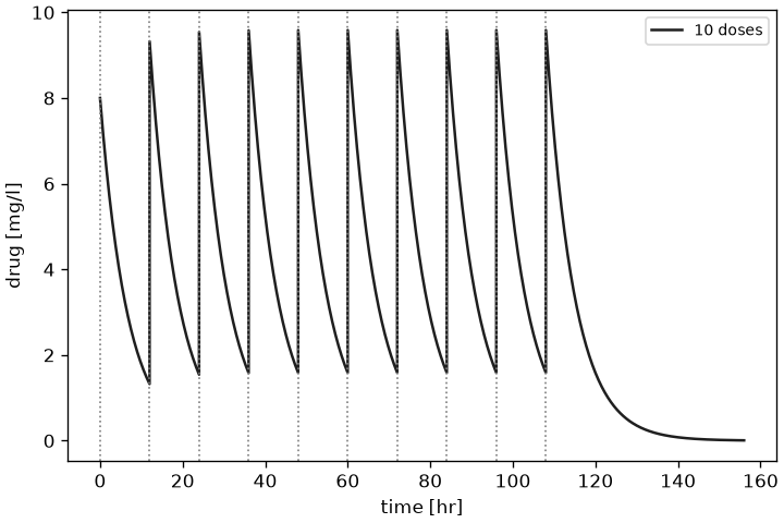
accumulation_ratio compares two analyses of the same dosing interval instead, the steady state study against a single dose study; with the result and the single curve of the snippet above:
from pkpdutils.nca import accumulation_ratio

first_dose = nca_single(single, options=NCAOptions(auc_method=AUCMethod.LOG, tau=12))
ratios = accumulation_ratio(result, first_dose)
print(float(ratios["accumulation_ratio"]))  # 1.1980336082689775
print(float(ratios["stationarity_ratio"]))  # 0.99999998477002
The second variable of that dataset is the stationarity ratio \(\mathrm{AUC}_{0\text{-}\tau}^\mathrm{ss} / \mathrm{AUC}_{0\text{-}\infty,\mathrm{obs}}^\mathrm{single}\) (CDISC SRAUC), 1 when the clearance did not change over the study.
The per-interval parameters (interval_*, NCAResult.intervals()), the steady state parameters of the last interval and the point parameters from the last dose on are all part of the one result. A batch is analysed the same way, and NCAOptions(tau=...) turns a single dose curve into a multiple dose analysis of one interval; the walk-through of a twice daily study is in Workflows.
An interval whose last sample falls short of its end
A study rarely samples exactly at the nominal end of the dosing interval, and a sample a few minutes early used to cost every steady state parameter of that profile. NCAOptions.tau_tolerance (0.1 of \(\tau\) by default) is how far the last measurable sample may fall short before the interval is given up: within it the exposure is completed with the terminal regression from \(t_\mathrm{last}\) to the end of the interval, the trough is that regression at the end, and auc_tau_extrap_fraction reports the share which was extrapolated2. The curve of the snippet above, cut half an hour before the end of its last interval:
# the same ten doses, but the last sample an hour before the end of the
# last interval, which is 8.3 % of tau and inside the tolerance
short = superposition(
    single, protocol, options=options, grid=np.arange(0.0, 119.1, 0.5)
)
completed = nca_single(short, options=options).to_quantities()
print(f"{completed['auc_tau']:~P}")
print(f"{completed['auc_tau_extrap_fraction']:~P}")
print(f"{completed['ctrough']:~P}")

# the same curve with the tolerance switched off
strict = nca_single(short, options=options.model_copy(update={"tau_tolerance": 0.0}))
print(float(strict["auc_tau"]), strict.flags())
53.33333252106773 h⋅mg/l
0.03204862198179163
1.584268987991663 mg/l
nan ['INCOMPLETE_INTERVAL', 'EXTRAPOLATED_TROUGH']
The completed interval carries the exposure of the whole interval, 3.2 % of it extrapolated, and the trough is the terminal regression at \(\tau\); with the tolerance switched off, or with a sample which falls further short, the parameters stay NaN and the sample is flagged INCOMPLETE_INTERVAL as before.
Time to steady state
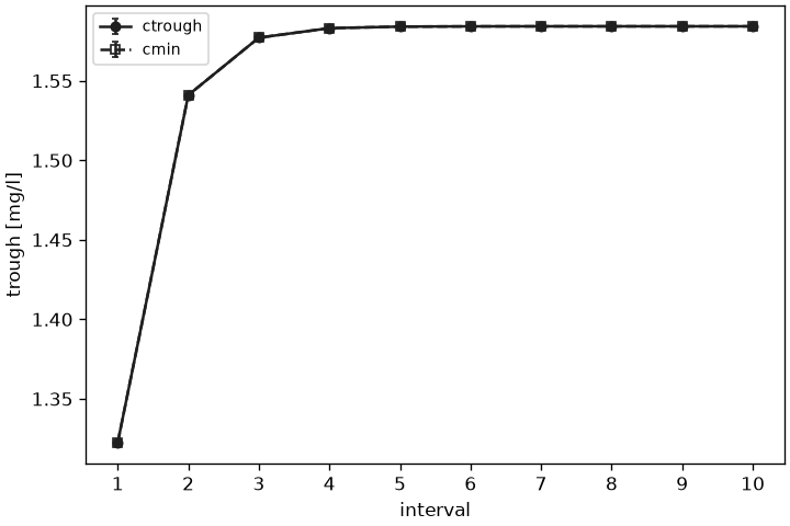
The trough of every dosing interval is in the result, so the time at which the troughs reach their plateau is a curve through them (pkpdutils.nca.tss). time_to_steady_state estimates it with the two methods of PKNCA13: "monoexponential" fits \(C_\mathrm{trough}(t) = C_\mathrm{ss}(1 - e^{-k t})\) and reports \(-\ln(1 - f) / k\), the time to the fraction \(f\) of the plateau, and "stepwise" regresses the troughs from every interval on and reports the start of the first interval whose trend is no longer significant. ICH M13A asks a study to "document appropriate dosage administration and sampling to demonstrate the attainment of steady-state"11, and this is that number.
from pkpdutils.nca import time_to_steady_state
from pkpdutils.plot import plot_troughs

estimate = time_to_steady_state(result, fraction=0.9)
print(estimate.method, round(float(estimate.tss), 3), round(float(estimate.c_ss), 3))
print(round(float(time_to_steady_state(result, method="stepwise").tss), 3))

plot_troughs(result, x="time").savefig("troughs.png", dpi=120)
The predicted curve accumulates with the terminal rate constant of the single dose curve, \(\lambda_z = 0.15\,\mathrm{h}^{-1}\), so 90 % of the plateau is reached after \(\ln 10 / \lambda_z = 15.35\) h, in the second dosing interval, and the plateau is the trough the intervals converge to, 1.584 mg/l. The stepwise estimate is 0: the troughs of a noiseless prediction carry no significant linear trend at all, which is the answer "already at steady state in the first interval". On measured data the stepwise estimate is the conservative one, since it only asks that the troughs stop rising. plot_troughs draws the troughs against the end of their interval, the figure of examples/steady_state.py:
Bioavailability
The fraction of a dose which reaches the circulation is the dose normalized exposure of a test treatment over that of a reference treatment (pkpdutils.nca.bioavailability), absolute against an intravenous reference and relative against any other6. bioavailability is the geometric mean ratio of the two dose normalized samples with its confidence interval, paired by subject in a crossover:
import numpy as np

from pkpdutils import Route, Timecourses
from pkpdutils.nca import bioavailability

subjects = ["s1", "s2", "s3", "s4"]
fractions = np.array([0.42, 0.55, 0.61, 0.70])
sampling = np.array([0.0, 0.25, 0.5, 0.75, 1, 1.5, 2, 3, 4, 6, 8, 12, 16, 24])
ke, ka, volume = 0.25, 1.2, 20.0


def crossover(values: np.ndarray, amount: float, route: Route) -> Timecourses:
    return Timecourses.from_arrays(
        sampling,
        values,
        time_unit="hr",
        unit="mg/l",
        dims=("individual",),
        coords={"individual": subjects},
        dose={"amount": np.full(len(subjects), amount), "unit": "mg"},
        route=route,
        substance="drug",
    )


# 100 mg intravenously, and 200 mg orally of which a fraction is absorbed
bolus = (100.0 / volume) * np.exp(-ke * sampling)
absorbed = (
    (200.0 / volume)
    * ka
    / (ka - ke)
    * (np.exp(-ke * sampling) - np.exp(-ka * sampling))
)
reference = nca(
    crossover(np.tile(bolus, (4, 1)), 100.0, Route.IV_BOLUS), options=options
)
test = nca(crossover(fractions[:, None] * absorbed, 200.0, Route.ORAL), options=options)

f = bioavailability(test, reference, dim="individual")
print(f"{f.name} {f.gmr:.3f} [{f.ci_low:.3f}, {f.ci_high:.3f}] ({f.ci_level:.0%})")
The four subjects absorb 42 % to 70 % of the oral dose and the estimate is the geometric mean of those fractions with the interval of four subjects around it. The reference is intravenous, so the ratio is the absolute bioavailability f_abs; against an extravascular reference the same call reports f_rel. parameter= selects the exposure to compare (auc_inf_obs by default, auc_last or auc_tau for a study which does not extrapolate), paired= overrides the pairing of a parallel design and reference_route= names the route of the reference when the result does not say which one it was.
Large batches are analysed in chunks of at most NCAOptions(chunk_rows=5000) rows, which bounds the memory of the vectorized core, and the chunks are mapped in order over the workers of NCAOptions(n_workers=...); both apply to the steady state path as well. The core is vectorized numpy and releases the GIL, so the workers are threads of the calling process (no if __name__ == "__main__": guard, no copy of the batch, a pool that starts in half a millisecond and is shared with every later call). The default n_workers=None decides by size: the calling thread up to 20 000 rows (pkpdutils.parallel.NCA_WORKER_THRESHOLD), where the analysis is faster than the pool, and one thread per usable core, at most 8, above it; n_workers=1 forces the serial run and n_workers=n uses that many threads. The rows are cut into about one chunk per worker, so a large batch keeps every thread busy, and the temporaries of the core live for as many chunks as run at once: a parallel run holds min(n_workers, n_chunks) * chunk_rows rows of them, not chunk_rows, which is what a large batch pays for its speed. Group timecourses with sd/se get uncertainty variables per parameter, individual results are summarized with NCAResult.summarize, see Uncertainty10; partial areas come from partial_auc, whose interval may start before the first sample of a curve but not before its dose: the value at the dose is then 0 for an extravascular dose and for an infusion and the back-extrapolated \(C_0\) for a bolus. The figures are described in Plotting, the examples are examples/nca_single.py, examples/nca_batch.py, examples/steady_state.py and examples/nca_from_sbmlsim.py, the reference of the modules is in API: nca.
References
-
Gabrielsson J, Weiner D. Pharmacokinetic and Pharmacodynamic Data Analysis: Concepts and Applications. 5th ed. Swedish Pharmaceutical Press; 2016. See References. ↩
-
Certara. Phoenix WinNonlin User's Guide: Noncompartmental Analysis. See References. ↩↩↩↩↩↩↩↩↩↩↩↩↩↩↩
-
Rowland M, Tozer TN. Clinical Pharmacokinetics and Pharmacodynamics. 4th ed. 2011, ch. 11. See References. ↩
-
Gabrielsson J, Weiner D. Non-compartmental analysis. Methods Mol Biol. 2012;929:377-389. See References. ↩
-
Bae KS. NonCompart: Noncompartmental Analysis for Pharmacokinetic Data. CRAN package. See References. ↩
-
U.S. Food and Drug Administration. Bioavailability Studies Submitted in NDAs or INDs - General Considerations. 2022. See References. ↩↩
-
Chiou WL. J Pharmacokinet Biopharm. 1978;6(6):539-546. See References. ↩
-
Yeh KC, Kwan KC. J Pharmacokinet Biopharm. 1978;6(1):79-98. See References. ↩
-
Purves RD. J Pharmacokinet Biopharm. 1992;20(3):211-226. See References. ↩
-
U.S. Food and Drug Administration. Population Pharmacokinetics. 2022. See References. ↩
-
International Council for Harmonisation. ICH M13A: Bioequivalence for Immediate-Release Solid Oral Dosage Forms. 2024. See References. ↩↩↩↩↩
-
U.S. Food and Drug Administration. Bioequivalence Studies With Pharmacokinetic Endpoints for Drugs Submitted Under an ANDA. 2026. See References. ↩
-
Denney W, Duvvuri S, Buckeridge C. Simple, automatic noncompartmental analysis: the PKNCA R package. J Pharmacokinet Pharmacodyn. 2015;42:S65. See References. ↩↩↩↩