Uncertainty¶

Published pharmacokinetic data are mostly group data²³: the mean concentration of a group at every sampling time with its standard deviation or standard error and the number of subjects. The parameters of the mean curve are point estimates; how uncertain they are depends on the uncertainty of the points and on how the parameters depend on them. pkpdutils propagates the uncertainty of a group timecourse to every parameter of the non-compartmental analysis by a parametric bootstrap or by the delta method, and it summarizes the parameters of individual curves over the individuals with the same set of variables, so that the statistics of the next pages accept both.

Concepts¶

Spread of the mean and spread of the individuals. The standard error \(\mathrm{se}_i = \mathrm{sd}_i / \sqrt{n_i}\) of a time point is the uncertainty of the group mean; the standard deviation \(\mathrm{sd}_i\) is the spread of the individual subjects. Which one to propagate depends on the question: the uncertainty of the parameters of the mean curve (BootstrapSpread.SE, the default) or the spread of the parameters over subjects (BootstrapSpread.SD). A Timecourse carries sd, se and n and derives the missing one; the result reports both x_se and x_sd, converting with \(\sqrt n\), and x_geocv is on the same between-subject scale as x_sd.

The two scales also decide what an interval means. x_ci_low/x_ci_high are always a confidence interval of the estimate: the percentile interval of the replicates under se draws, and the normal approximation \(x \pm z\,\mathrm{se}(x)\) (on the log scale for log-normal parameters) under sd draws, whose replicates are individual curves rather than replicates of the mean. The percentiles of those individual replicates are reported separately as x_pi_low/x_pi_high: they bound the individuals, not the estimate, and are therefore about \(\sqrt n\) times wider.

Bootstrap. The parametric bootstrap ¹ draws every time point of the curve from a distribution with the observed mean and spread, analyses every replicate curve as if it were observed, and reads the uncertainty of a parameter from the spread of its replicates. Normal draws (the default) are set to 0 when they fall below 0 for concentrations, which cannot be negative; this biases a point whose relative spread is large upwards, so BootstrapDistribution.LOGNORMAL, which has the same mean and spread and is positive by construction, is the better choice there. Effect timecourses (Kind.EFFECT) are not clipped, because their values are legitimately negative, and they reject log-normal draws for the same reason. n_boot replicates of every curve run through the same vectorized code as the curves themselves, so the bootstrap of a batch is one call; the draws \((N, B, n_\mathrm{time})\) are materialized before that call, and NCAOptions.chunk_rows bounds the memory of the vectorized core, not of the draws.

Under se draws the interval is the percentile interval of the replicates, which is asymmetric around the estimate for a strongly non-linear parameter (lambda_z, mrt) and is not guaranteed to contain it.

Delta method. The delta method ¹ linearizes a parameter around the observed curve: every time point is perturbed by a small step, the numerical derivative of every parameter with respect to every point is formed, and the variances of the points add through the squared derivatives⁴. It costs one analysis per time point instead of one per replicate, gives symmetric normal intervals (log-normal parameters on the logarithmic scale) and is exact for the linear trapezoid area; it cannot follow a change of the terminal window. A perturbation which selects a different window (lambda_z_n_points or lambda_z_t_first changes) turns the difference quotient into a jump between two regressions, which inflated the standard error of every terminal parameter; such points are skipped for the parameters which depend on the terminal phase and the sample carries NCAFlag.DELTA_WINDOW_CHANGE, which says that their uncertainty is incomplete. Use the bootstrap, which follows the window, for those samples.

Discrete parameters. tmax, tlast, tmin, tmax_half, temax and the counts of the terminal regression are read from the observed points; they carry no uncertainty variables. The regression diagnostics (lambda_z_stderr, lambda_z_r2, lambda_z_r2_adj, lambda_z_intercept) carry no uncertainty variables either.

Individuals. When every subject has its own curve the parameters of the subjects are a sample: NCAResult.summarize(dim) reduces the result over a sample dimension to the mean, standard deviation, standard error, the coefficient of variation x_cv (\(\mathrm{sd}/\lvert \bar x \rvert\), a fraction), a t-based confidence interval of the mean, median, quartiles, x_min and x_max, the number of values and, for log-normal parameters, the geometric mean and geometric CV. The per-interval parameters of a multiple dose analysis (interval_*) are reduced over the subjects as well and keep their interval dimension, so that the mean trough per dosing interval is one call; summary_table formats the whole set into the parameter table of a publication, see NCA. The variables have the same names as the bootstrap output, so a group result and a summary look alike. The two counts of a summary differ: n is the number of samples along the reduced dimension, x_n the number of them at which x is finite, and every statistic of x uses x_n (\(\mathrm{se} = \mathrm{sd}/\sqrt{x_n}\), the interval uses \(t\) with \(x_n - 1\) degrees of freedom). A parameter which does not apply to every subject, such as lambda_z without a terminal phase, therefore has \(x_n < n\).

Which path an analysis takes follows from what the batch carries, and all three end in the same variables:

flowchart TD
  Q{"what does the batch carry?"}
  Q -->|"mean + sd/se + n<br/>(a group curve)"| G["NCAOptions.resolve_uncertainty"]
  Q -->|"one curve per subject"| I["nca over the individual dimension"]
  G --> B["bootstrap (the default)<br/>resample_values -> N*B rows<br/>run_rows -> reduce_replicates"]
  G --> D["delta<br/>perturb every point once,<br/>numerical Jacobian"]
  B --> SPREAD{"BootstrapSpread"}
  SPREAD -->|SE| CI1["x_se, percentile x_ci_low/high"]
  SPREAD -->|SD| CI2["x_sd, normal x_ci_low/high<br/>+ x_pi_low/high (individuals)"]
  D --> CI3["x_se, symmetric normal interval<br/>flag DELTA_WINDOW_CHANGE"]
  I --> S["NCAResult.summarize(dim)<br/>mean, sd, se, cv, t interval,<br/>median, q25, q75, min, max, x_n"]
  CI1 --> V["the same variable names:<br/>x, x_sd, x_se, x_ci_low, x_ci_high,<br/>x_geomean, x_geocv, n"]
  CI2 --> V
  CI3 --> V
  S --> V

Math¶

Parametric bootstrap with \(B\) replicates of a point \(\bar C_i\) with spread \(s_i\):

Delta method with the step \(h_i = \delta\, \mathrm{se}_i\):

For the linear trapezoid rule \(\mathrm{AUC} = \sum_i w_i C_i\) is linear in the points and the delta method is exact: \(\mathrm{Var}(\mathrm{AUC}) = \sum_i w_i^2 \mathrm{se}_i^2\).

Summary of \(n\) individual values \(x_j\): mean \(\bar x\), \(\mathrm{sd}\) with \(n-1\), \(\mathrm{se} = \mathrm{sd}/\sqrt n\), \(\mathrm{CI} = \bar x \pm t_{n-1,\,1-\alpha/2}\,\mathrm{se}\), geometric mean and CV from \(\ln x_j\).

Variables¶

API¶

Group data: the bootstrap is the default as soon as the timecourse carries sd or se:

from pkpdutils import (
    BootstrapDistribution,
    BootstrapSpread,
    Dose,
    NCAOptions,
    Route,
    Timecourse,
    UncertaintyMethod,
    nca_single,
)

group = Timecourse(
    time=[0.5, 1, 2, 4, 8, 12, 24],
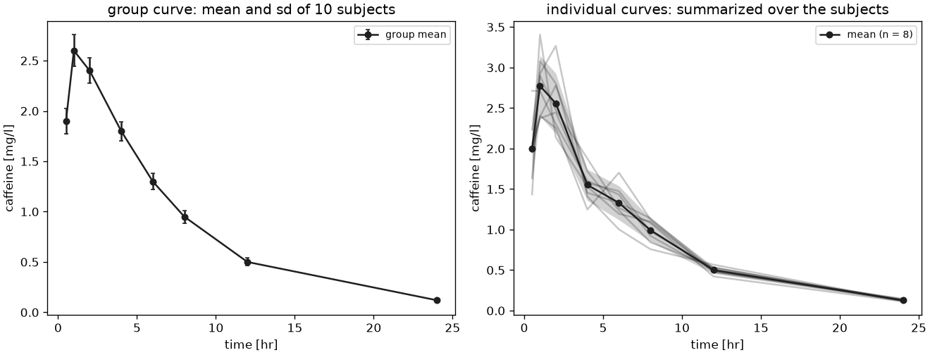
    value=[1.9, 2.6, 2.4, 1.8, 0.95, 0.5, 0.12],
    sd=[0.4, 0.5, 0.4, 0.3, 0.2, 0.12, 0.04],
    n=10,
    time_unit="hr",
    unit="mg/l",
    dose=Dose(amount=100, unit="mg", route=Route.ORAL),
    substance="caffeine",
)
result = nca_single(group, options=NCAOptions(seed=1, n_boot=2000))
q = result.to_quantities()
print(f"auc  {q['auc_inf_obs']:~P}")
print(f"se   {q['auc_inf_obs_se']:~P}")
print(f"ci   {q['auc_inf_obs_ci_low']:~P} - {q['auc_inf_obs_ci_high']:~P}")

# the spread of the individuals instead of the uncertainty of the mean
spread = nca_single(
    group,
    options=NCAOptions(
        seed=1,
        bootstrap_spread=BootstrapSpread.SD,
        bootstrap_distribution=BootstrapDistribution.LOGNORMAL,
    ),
)
print(f"sd   {spread.to_quantities()['auc_inf_obs_sd']:~P}")

# the delta method, one analysis per time point instead of one per replicate
delta = nca_single(group, options=NCAOptions(uncertainty=UncertaintyMethod.DELTA))
print(f"se   {delta.to_quantities()['auc_inf_obs_se']:~P} (delta)")

auc  19.99379796863043 h⋅mg/l
se   0.5510537013864025 h⋅mg/l
ci   18.977328445090134 h⋅mg/l - 21.062905318509465 h⋅mg/l
sd   1.762755309648389 h⋅mg/l
se   0.5480678838283282 h⋅mg/l (delta)

The bootstrap and the delta method agree on the standard error of an area, which is linear in the points; the standard deviation over the individuals is about \(\sqrt{10}\) times the standard error of the mean, the two scales the concepts above describe.

Individual curves: the parameters of the subjects are a sample and summarize reduces them over the sample dimension.

import numpy as np

from pkpdutils import Dose, Route, Timecourses, nca, partial_auc

time = np.array([0.5, 1, 2, 4, 8, 12, 24])
rng = np.random.default_rng(7)
ke = rng.uniform(0.12, 0.25, size=8)
values = np.stack(
    [2.6 * np.exp(-k * time) * rng.lognormal(0, 0.05, time.size) for k in ke]
)
individuals = Timecourses.from_arrays(
    time,
    values,
    time_unit="hr",
    unit="mg/l",
    dims=("individual",),
    coords={"individual": [f"s{i + 1}" for i in range(8)]},
    dose=Dose(amount=100, unit="mg", route=Route.ORAL),
    substance="drug",
)
result = nca(individuals)
summary = result.summarize("individual")
print(
    summary.to_dataframe()[
        [
            "auc_inf_obs",
            "auc_inf_obs_sd",
            "auc_inf_obs_se",
            "auc_inf_obs_geocv",
            "auc_inf_obs_n",
            "n",
        ]
    ].to_string(index=False)
)
# the formatted table of the same statistics
print(
    result.summary_table("individual", parameters=["auc_inf_obs", "thalf"]).to_string(
        index=False
    )
)

# a partial area of every sample, here AUC(0.5-6)
area = partial_auc(individuals, 0.5, 6.0)
print(area.values.round(3), area.attrs["units"])

 auc_inf_obs  auc_inf_obs_sd  auc_inf_obs_se  auc_inf_obs_geocv  auc_inf_obs_n   n
   12.822918        3.908277        1.381785           0.287253            8.0 8.0
  parameter                     unit n mean   sd     cv geomean  geocv median  min  max
auc_inf_obs hour * milligram / liter 8 12.8 3.91 30.5 %    12.4 28.7 %   11.0 9.20 20.4
      thalf                     hour 8 3.79 1.00 26.5 %    3.68 24.9 %   3.28 2.98 5.72
[7.872 6.731 7.344 8.679 8.781 7.204 9.88  7.364] hour * milligram / liter

The two paths of examples/group_uncertainty.py: the reported group curve, whose spread the bootstrap and the delta method propagate, and the individual curves, whose parameters are summarized over the subjects.

partial_auc(batch, t_start, t_end, *, options=...) is the area between two times of every sample, as in the snippet above; the interval may start before the first sample of a curve but not before its dose.

The example is examples/group_uncertainty.py; the reference of the module is in API: nca.uncertainty.

References¶