Pharmacodynamics¶

A pharmacodynamic timecourse measures an effect over time, a concentration-effect relationship measures the effect against the concentration. pkpdutils treats both with the tools of the previous pages: effect timecourses go through the non-compartmental analysis with Kind.EFFECT, concentration-effect data are fitted with the Emax family of the curve fitting.

Effect timecourses¶

NCAOptions(kind=Kind.EFFECT) switches the analysis to effect parameters: the baseline e0 (the first value), the observed maximum emax_obs and its time temax, the area under the effect curve auec_last (linear trapezoids, any sign) to the time of the last valid point tlast, the baseline corrected auec_baseline and emax_baseline, and, with effect_threshold, the time the linearly interpolated curve spends above the threshold, time_above. No terminal phase and no dose parameters are computed. The areas are always linear trapezoids: the logarithmic rules are exact for the mono-exponential decline of a concentration and need positive values, which an effect does not have, so auc_method does not apply here; lloq and blq do apply and work as they do for a concentration, the sample being flagged BLQ_TRUNCATED. Group effect curves with sd/se get the same uncertainty variables as concentrations (Uncertainty); their bootstrap draws are not clipped at 0, because an effect is legitimately negative, for the same reason log-normal draws are rejected.

import numpy as np

from pkpdutils import Kind, NCAOptions, Timecourse, nca_single

# an effect over time: a baseline of 10, a maximum around two hours
time = np.array([0.0, 0.5, 1, 2, 3, 4, 6, 8, 12])
effect = 10 + 12 * (np.exp(-0.2 * time) - np.exp(-1.5 * time))
tc = Timecourse(
    time=time,
    value=effect,
    time_unit="hr",
    unit="mmHg",
    substance="effect",
)
result = nca_single(tc, options=NCAOptions(kind=Kind.EFFECT, effect_threshold=15.0))
q = result.to_quantities()
for name in (
    "e0",
    "emax_obs",
    "temax",
    "emax_baseline",
    "auec_last",
    "auec_baseline",
    "time_above",
):
    print(f"{name:<14} {q[name]:~P}")

e0             10.0 mmHg
emax_obs       17.446395732013304 mmHg
temax          2.0 h
emax_baseline  7.446395732013304 mmHg
auec_last      166.56834496993235 h⋅mmHg
auec_baseline  46.56834496993237 h⋅mmHg
time_above     3.9323708621578644 h

Effect intervals¶

An effect timecourse carrying a dosing protocol of more than one dose gets the same multiple dosing analysis as a concentration timecourse (Non-compartmental analysis, "Multiple dosing"): every dosing interval reports interval_auec, interval_emax, interval_temax, interval_emin, interval_eavg and, with effect_threshold, interval_time_above (NCAResult.intervals()), and the last complete interval reports the steady state parameters auec_tau, emin_ss, emax_ss, eavg, time_above_tau, accumulation_ratio_obs, n_doses and tau. The baseline e0, the observed maximum emax_obs/temax and the baseline corrected variables are computed from the last dose on, the same reference dose rule as a concentration timecourse.

# not executed
# `tc_protocol`: an effect timecourse carrying a `Dosing` of several doses,
# built like the curve above but with `dosing=Dosing.regimen(...)`
result = nca_single(
    tc_protocol,
    options=NCAOptions(kind=Kind.EFFECT, effect_threshold=15.0),
)
result.intervals()[["interval", "interval_auec", "interval_emax"]]
result.to_quantities()["auec_tau"]  # the last, complete interval

Concentration-effect relationships¶

The Emax model describes a saturable effect, the Hill coefficient \(n\) of the sigmoid form makes the transition steeper, and the Imax forms describe inhibition ¹²³:

\(E_0\) is the effect without drug, \(E_\mathrm{max}\) the maximal effect above it, \(\mathrm{EC}_{50}\) the concentration of half-maximal effect and \(\mathrm{EC}_{90}\) the concentration of 90 % of it; \(I_\mathrm{max}\) is a fraction between 0 and 1, so the inhibited effect is \(E_0(1 - I_\mathrm{max})\) at saturation. The models are fitted with the curve fitting engine, which reports the standard errors and confidence intervals of the parameters and of \(\mathrm{EC}_{90}\); compare_models decides between Emax, sigmoid Emax and a linear relationship by AICc, which with few concentrations often keeps the simpler model. The same models describe a pharmacokinetic parameter against the dose of a perpetrator, for example Imax for a clearance against the dose of an inhibitor.

import numpy as np

from pkpdutils import Emax, FitOptions, Linear, SigmoidEmax, compare_models, fit

# the effect at eight concentrations, e0 = 5, emax = 40, ec50 = 12, hill = 1.6
rng = np.random.default_rng(3)
concentration = np.array([0.5, 1, 2, 5, 10, 20, 50, 100.0])
effect = 5 + 40 * concentration**1.6 / (12.0**1.6 + concentration**1.6)
effect = effect + rng.normal(0, 1.0, concentration.size)

result = fit(
    SigmoidEmax(),
    concentration,
    effect,
    x_unit="ng/ml",
    y_unit="mmHg",
    options=FitOptions(n_starts=10, seed=0),
)
q = result.to_quantities()
for name in ("e0", "emax", "ec50", "hill", "ec90"):
    print(f"{name:<5} {q[name]:~P}")
print(f"ec90 95 % interval {q['ec90_ci_low']:~P} - {q['ec90_ci_high']:~P}")

comparison = compare_models(
    [Emax(), SigmoidEmax(), Linear()],
    concentration,
    effect,
    x_unit="ng/ml",
    y_unit="mmHg",
)
print(
    comparison.table[["model", "aicc", "delta_aicc", "akaike_weight"]].to_string(
        index=False
    )
)
print("best:", comparison.best.item())

e0    5.0646456598207035 mmHg
emax  38.73988957163847 mmHg
ec50  11.977716913982151 ng/ml
hill  1.643997431701769
ec90  45.5842101424971 ng/ml
ec90 95 % interval 3.6372317046843747 ng/ml - 87.53118858030982 ng/ml
       model      aicc  delta_aicc  akaike_weight
        emax 31.418000    0.000000       0.996360
sigmoid_emax 43.834014   12.416013       0.002006
      linear 44.244300   12.826299       0.001634

The sigmoid model recovers the parameters the data was built from, but with eight concentrations the plain Emax wins the comparison by a wide margin: the Hill coefficient costs a parameter and an AICc penalty which this much data does not pay for, which is why the interval of \(\mathrm{EC}_{90}\) is so wide.

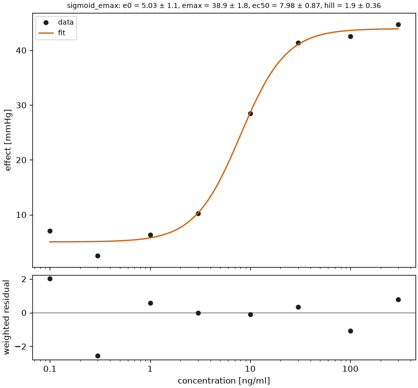
The example is examples/emax.py, the figures are described in Plotting and the reference of the models is in API: fit.models.

References¶