Urinary excretion¶

A urine study does not sample a concentration over time. The urine of a subject is collected over intervals, the volume of every collection is recorded and the substance is measured in it, and the question is how much of the dose left the body unchanged and how fast. pkpdutils.nca.urine reads such a study as an Excretion and analyses it as the excretion rate curve, the convention of every tool in the field, so that the machinery of the non-compartmental analysis applies unchanged: the same trapezoid rules, the same terminal regression, the same result container. The renal clearance, which Phoenix WinNonlin, PKanalix and Pumas all leave to the user, is part of the result.

Concepts¶

Collection intervals. A collection is an interval \([s_k, e_k]\) with a volume \(V_k\) and either the concentration \(c_k\) measured in it or the amount \(A_k = c_k V_k\) it contains. The intervals are sorted by their start, are strictly increasing and may not overlap; a gap between two of them is allowed, since a subject does not void continuously. The concentration is given in unit / volume_unit: with unit="mg" and volume_unit="ml" it is in mg/ml, because the amount of a collection is the concentration times the volume and nothing else converts between them.

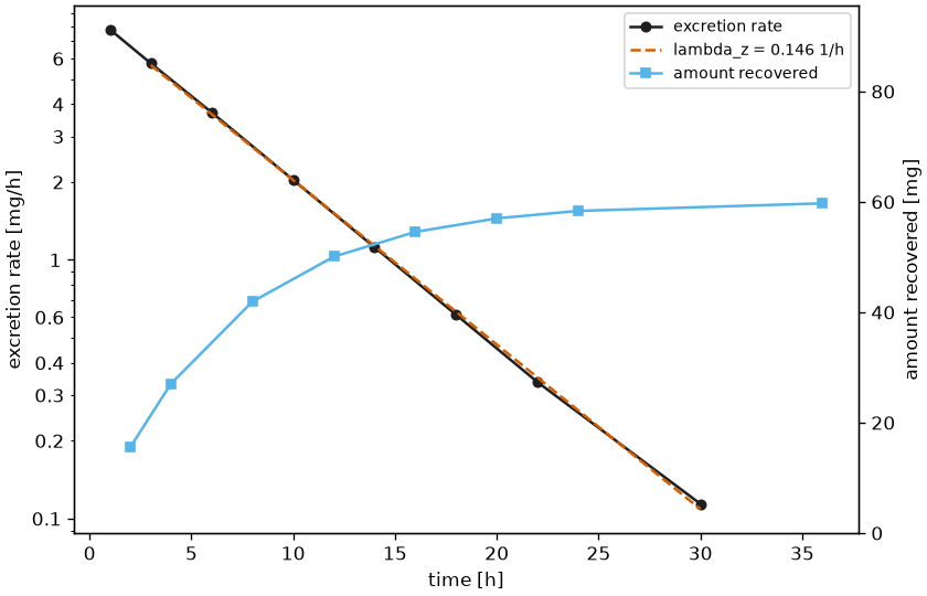
The excretion rate curve. The amount of a collection belongs to the whole interval, not to a time, so it is reported as the rate \(\dot A_k = A_k / (e_k - s_k)\) at the midpoint \(\bar t_k = (s_k + e_k) / 2\) of its interval. This curve behaves like a concentration curve: it rises to a maximum (max_rate at tmax_rate), falls log-linearly in the terminal phase and its area is an amount. Phoenix WinNonlin¹ analyses urine in its models 210 to 212, which mirror the plasma models 200 to 202 exactly, and nca_urine runs the same core (compute_parameters) on the rate curve, which is why the parameters are the plasma ones under the names of the field: aurc_last is the auc_last of the rate curve, mid_pt_last its tlast, rate_last its clast.

The value at the dose follows the route, as it does for a concentration curve: 0 after an extravascular dose, the back-extrapolated rate after an intravenous bolus (NCAOptions.c0_method) and none without a dose, in which case the area starts at the first midpoint.

What was recovered. The rate curve is a model of the excretion; the amount recovered is not. amount_recovered is the plain sum \(A_e = \sum_k A_k\) of the collections, percent_recovered that amount as a percentage of the dose and vol_ur the volume collected. EMA CPMP/EWP/QWP/1401/98 Rev. 1² asks for exactly this: "When using urinary data, Ae(0-t) and, if applicable, Rmax should be determined", both analysed against the 80.00 to 125.00 % interval of a bioequivalence study.

Renal clearance. With the plasma curve of the same subject the renal clearance is the recovered amount over the plasma exposure of the window it was recovered in. Giving the plasma curve integrates it over the collection span \([s_1, e_K]\) (partial_auc), which is the window the amount belongs to; giving the NCAResult of that curve takes its auc_last instead, which is the same window only when the curve ends with the last collection.

Only auc_method, c0_method, terminal and extrapolation_warning of NCAOptions are read. The rules which read a concentration - lloq, blq, kind, partial_aucs, acceptance, the uncertainty - do not apply to a rate curve and are ignored.

Math¶

The rate of a collection and the time it is reported at:

The areas under the rate curve, with the trapezoid rule of options.auc_method and the terminal regression \(\ln \dot A = b - \lambda_z t\) of the last points of the curve:

The recovery and the renal clearance:

\(\lambda_z\) of the rate curve is the elimination rate constant of the substance whenever the renal elimination follows the plasma, which is what makes the half-life of a urine study comparable with the half-life of the plasma curve. The rate of a collection is the average rate over its interval, not the instantaneous rate at its midpoint; the two differ by \(\sinh(\lambda_z d / 2) / (\lambda_z d / 2)\) with the length \(d\) of the interval, a factor of the interval length alone, so the slope is unbiased as long as the collections have the same length and the bias is second order in \(\lambda_z d\) otherwise.

Results¶

nca_urine returns an NCAResult without sample dimensions (one subject), with the rate curve as the point variables rate and midpoint over the dimension collection.

The names follow Phoenix WinNonlin¹ and PKanalix; the CDISC codelist calls them AURCLST, AURCIFO, RCAMINT, RCPCINT, VOLPK and RENALCL.

API¶

import numpy as np

from pkpdutils import Dose, Excretion, Route, nca_urine

# eight collections after a 100 mg oral dose, the amount measured in each
excretion = Excretion(
    start=[0.0, 2.0, 4.0, 8.0, 12.0, 16.0, 20.0, 24.0],
    end=[2.0, 4.0, 8.0, 12.0, 16.0, 20.0, 24.0, 36.0],
    amount=[9.8, 11.6, 14.9, 8.2, 4.5, 2.5, 1.4, 1.4],
    volume=[180.0, 150.0, 260.0, 240.0, 210.0, 190.0, 220.0, 360.0],
    unit="mg",
    volume_unit="ml",
    time_unit="hr",
    dose=Dose(amount=100.0, unit="mg", route=Route.ORAL),
    substance="drug",
    label="S1",
)
print(np.round(excretion.midpoint, 1))
print(np.round(excretion.rate, 2))

result = nca_urine(excretion)
q = result.to_quantities()
for name in ("max_rate", "tmax_rate", "mid_pt_last", "aurc_last", "aurc_inf_obs"):
    print(f"{name:<17} {q[name]:.4g~P}")
for name in ("lambda_z", "thalf", "amount_recovered", "percent_recovered", "vol_ur"):
    print(f"{name:<17} {q[name]:.4g~P}")

[ 1.  3.  6. 10. 14. 18. 22. 30.]
[4.9  5.8  3.72 2.05 1.12 0.62 0.35 0.12]
max_rate          5.8 mg/h
tmax_rate         3 h
mid_pt_last       30 h
aurc_last         49.14 mg
aurc_inf_obs      49.97 mg
lambda_z          0.1414 1/h
thalf             4.901 h
amount_recovered  54.3 mg
percent_recovered 54.3 %
vol_ur            1.81 l

The plasma curve of the same subject adds the renal clearance:

from pkpdutils import Timecourse

plasma = Timecourse(
    time=[0.0, 0.5, 1.0, 2.0, 4.0, 8.0, 12.0, 24.0, 36.0],
    value=[0.0, 1.85, 2.71, 3.18, 2.46, 1.32, 0.71, 0.11, 0.02],
    time_unit="hr",
    unit="mg/l",
    dose=Dose(amount=100.0, unit="mg", route=Route.ORAL),
    substance="drug",
    tissue="plasma",
)
renal = nca_urine(excretion, plasma=plasma)
print(f"clr {renal.to_quantities()['clr']:.4g~P}")

clr 2.096 l/h

plot_excretion draws the figure a mass balance study is read from: the rate curve with its terminal regression on a logarithmic axis and the amount recovered on a second axis, which flattens out as the excretion stops.

# not executed
from pkpdutils.plot import plot_excretion

plot_excretion(result, excretion).savefig("urine.png", dpi=120)

The example is examples/urine.py, the reference of the module is in API: nca.urine and the sparse designs of a preclinical study are in Sparse sampling.

References¶