Sparse sampling¶

A preclinical study rarely samples one animal repeatedly: the animal is sacrificed for its sample (a destructive design, one sample per animal) or contributes a few samples out of the schedule (a batch design). There is no curve per animal then, only a mean curve over the animals of every nominal time, and the exposure of the study is the area under that mean curve. pkpdutils.nca.sparse estimates it with the standard error of Bailer¹, the degrees of freedom of Nedelman, Gibiansky and Lau² and, for a batch design, the extension of Nedelman and Jia³ in the form Holder⁴ gives it, so the area of a toxicokinetic study comes with an interval rather than as a bare number. It is the design ICH S3A⁶ describes and the one every comparable tool supports (Phoenix WinNonlin models 200 to 202 and 210 to 212 with SE_AUClast, PKanalix since 2024R1, PKNCA sparse_auclast, the R package PK).

Concepts¶

The design as a matrix. The data is one row per animal and one column per nominal time, NaN where the animal has no sample at that time. A serial design has one finite value per row, a batch design several; the same matrix describes both and design="serial" is the promise that every row carries a single sample, which is checked.

Nominal times. The mean of a time point only exists at a nominal time, so the nominal schedule is used and never the actual sampling times, the caution Phoenix⁵ states for its sparse models. An animal sampled at 2.1 h instead of 2 h contributes to the mean of the nominal 2 h.

Why the trapezoid rule has to be linear. The area is a fixed linear combination of the means, \(\widehat{\mathrm{AUC}} = \sum_j w_j \bar y_j\), and that is exactly what makes its variance computable from the variances of the means. The logarithmic trapezoid rules are not linear in the values and have no variance of this kind, so the weights are always those of the linear rule and options.auc_method is not read.

What the area covers. The weights run over the nominal times as they are given, from the first of them, and nothing is inserted at time 0: an inserted point has no variance and would break the estimator. A design whose area is to start at the dose carries a nominal time 0 of its own, with the value 0 after an extravascular dose. auc_last ends at the last nominal time whose mean is positive, auc_all at the last nominal time with a sample.

One identity for every design. Written per animal instead of per time point the estimator is \(\widehat{\mathrm{AUC}} = \sum_i A_i\) with \(A_i = \sum_{j \in T_i} (w_j / n_j)\, y_{ij}\) over the times \(T_i\) the animal was sampled at. The animals are independent whatever the design, so the variance is a sum over the animals and is estimated batch by batch, a batch being the animals with the same sampling times. With one sample per animal a batch is one time point and the sum is Bailer's formula; with several it carries the covariances of Holder without ever forming them. A batch of a single animal has no variance of its own: the standard error is then NaN and the analysis logs why.

Math¶

The weights of the linear trapezoid rule over the \(J\) nominal times of the area:

The estimator and, for a serial design, the variance of Bailer¹ with the degrees of freedom of Nedelman, Gibiansky and Lau²:

The same numbers from the per-animal form, which is what is implemented and which covers the batch design of Nedelman and Jia³ and Holder⁴ as well:

with \(m_b\) animals in batch \(b\) and \(s^2_{A,b}\) the sample variance of their \(A_i\). Expanding that sample variance gives the covariance form,

with \(n_{jk}\) the animals sampled at both times and \(s_{jk}\) their sample covariance, which is 0 in a serial design. The interval of the area is the \(t\) interval \(\widehat{\mathrm{AUC}} \pm t_{1-\alpha/2,\nu}\,\mathrm{se}\), and the peak of the mean curve carries the standard error \(s_j/\sqrt{n_j}\) of the mean at its own time point, the SE_Cmax of Phoenix⁵.

Results¶

nca_sparse returns an NCAResult without sample dimensions (one mean curve), sparse_mean the mean curve itself as a Timecourses of one sample.

The mean curve of sparse_mean carries value, sd, se and n per time point, so it plots, prints and travels like any other group curve of the package, see Timecourses.

API¶

A serial design of 24 mice, four sacrificed at every nominal time:

import numpy as np

from pkpdutils import nca_sparse, sparse_mean

times = np.array([0.5, 1.0, 2.0, 4.0, 8.0, 12.0])
# one row per animal, NaN where the animal has no sample
values = np.full((24, 6), np.nan)
values[0:4, 0] = [41.0, 52.3, 45.8, 50.1]
values[4:8, 1] = [58.6, 79.2, 71.4, 82.5]
values[8:12, 2] = [66.7, 83.1, 74.5, 78.9]
values[12:16, 3] = [49.2, 64.4, 55.7, 62.8]
values[16:20, 4] = [16.1, 22.4, 19.8, 20.9]
values[20:24, 5] = [8.4, 13.2, 11.5, 12.0]

curve = sparse_mean(times, values, time_unit="hr", unit="ng/ml", substance="drug")
print(np.round(curve.values.reshape(-1), 2))
print(np.round(curve.ds["se"].to_numpy().reshape(-1), 2))

result = nca_sparse(times, values, design="serial", time_unit="hr", unit="ng/ml")
q = result.to_quantities()
for name in ("auc_last", "auc_last_se", "auc_last_df", "cmax", "cmax_se", "tmax"):
    print(f"{name:<12} {q[name]:.4g~P}")
print(result["n_animals"].to_numpy())

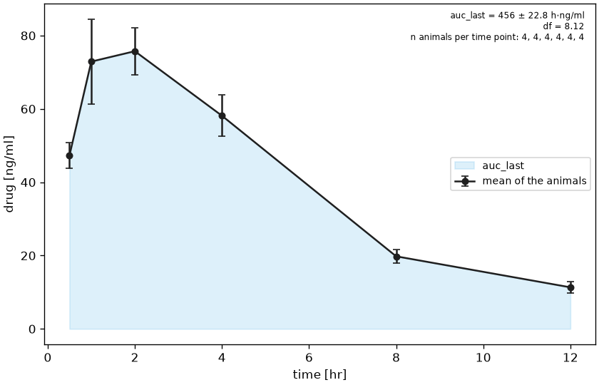
[47.3  72.93 75.8  58.03 19.8  11.28]
[2.5  5.31 3.5  3.5  1.34 1.02]
auc_last     456 h⋅ng/ml
auc_last_se  13.68 h⋅ng/ml
auc_last_df  7.506
cmax         75.8 ng/ml
cmax_se      3.505 ng/ml
tmax         2 h
[4 4 4 4 4 4]

The degrees of freedom are what the standard error is for: the interval of the area is a \(t\) interval, not a normal one, and with six time points of four animals it has about seven and a half degrees of freedom rather than 23.

from scipy.stats import t as student_t

auc = float(result["auc_last"])
se = float(result["auc_last_se"])
df = float(result["auc_last_df"])
half = student_t.ppf(0.975, df) * se
print(
    f"AUC = {auc:.1f} [{auc - half:.1f}, {auc + half:.1f}] {result.units('auc_last')}"
)

AUC = 456.0 [424.1, 487.9] hour * nanogram / milliliter

The same study as a batch design: twelve animals, each sampled at three of the six times. design="batch" adds the covariance between the time points an animal is shared by.

batch = np.full((12, 6), np.nan)
# batch A is sampled at 0.5, 2 and 8 hr, batch B at 1, 4 and 12 hr
batch[0:6, 0] = [41.0, 52.3, 45.8, 50.1, 47.7, 43.9]
batch[0:6, 2] = [66.7, 83.1, 74.5, 78.9, 76.2, 70.4]
batch[0:6, 4] = [16.1, 22.4, 19.8, 20.9, 20.1, 17.6]
batch[6:12, 1] = [58.6, 79.2, 71.4, 82.5, 74.0, 66.1]
batch[6:12, 3] = [49.2, 64.4, 55.7, 62.8, 58.3, 52.5]
batch[6:12, 5] = [8.4, 13.2, 11.5, 12.0, 11.8, 9.9]

paired = nca_sparse(times, batch, design="batch", time_unit="hr", unit="ng/ml")
for name in ("auc_last", "auc_last_se", "auc_last_df"):
    print(f"{name:<12} {paired.to_quantities()[name]:.4g~P}")

auc_last     449.8 h⋅ng/ml
auc_last_se  13.56 h⋅ng/ml
auc_last_df  8.904

plot_sparse draws the mean curve with its standard errors, the area shaded under the polygon the trapezoid rule integrates, and the estimate with the number of animals behind every time point.

# not executed
from pkpdutils.plot import plot_sparse

plot_sparse(curve, result).savefig("sparse.png", dpi=120)

The example is examples/sparse.py, the reference of the module is in API: nca.sparse. A group curve whose sd is known rather than a design of single samples is propagated differently, see Uncertainty.

References¶